import sympy as sp                                       # Symbolical math tools
import numpy as np                                       # Numerical math tools
import matplotlib.pyplot as plt # Visualization tools9 Paper work example
9.1 Problem
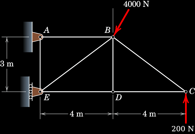
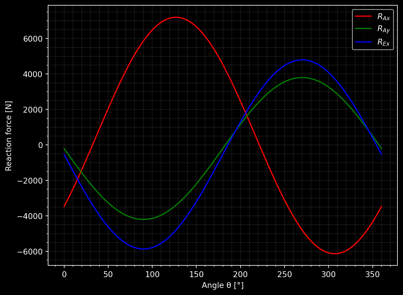
Determine how all of the forces in the system varies as the direction of the 4000 N force changes. 
9.2 Paperwork
This is an example of the minimal amount of “paperwork” necessary before you start working with Python.
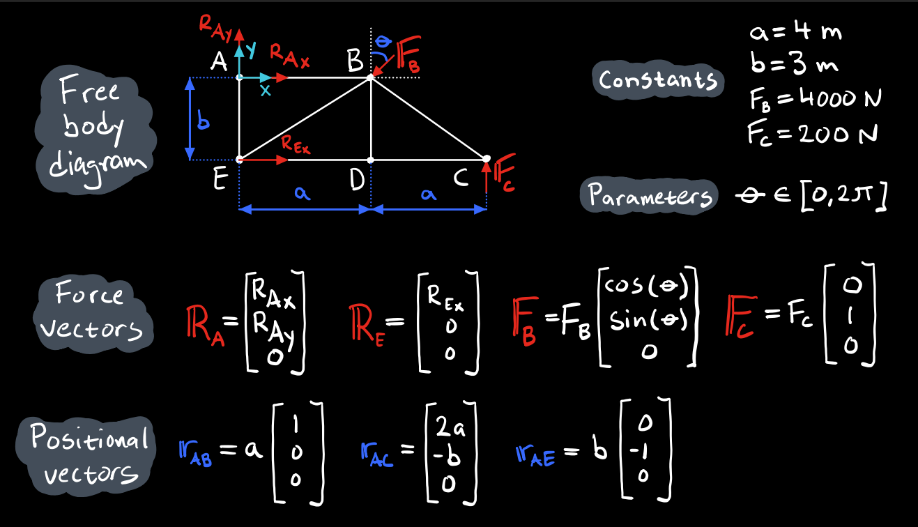
9.2.1 Free body diagram and vector definitions
A free body diagram consists of several definitions: a coordinate system, points of interest, forces, moments and distances. Additionally, clearly define any known constants or other parameters that are allowed to vary. Finally, define all force- and positional vectors in terms of both knowns and unknowns. 
9.2.2 Analysis of unknowns and equations of motion
Compare the number of unknown variables to the number of equations you can establish for the given problem. If they are the same, you can proceed to coding. If not, more thinking and/or paperwork is required! 
9.3 Code
9.3.1 Imports
9.3.2 Constants
a = 4                                                    # [m] Distance ED
b = 3                                                    # [m] Distance AE
F_B = 4000                                               # [N] Force magnitude: B
F_C = 200                                                # [N] Force magnitude: C
9.3.3 Parameters
theta = sp.symbols('theta', real=True) # [rad] Angle at B9.3.4 Variables
R_Ax, R_Ay, R_Ex = sp.symbols('R_Ax, R_Ay, R_Ex', real=True) # [N] Unknowns9.3.5 Force vectors
RR_A = sp.Matrix([R_Ax, R_Ay, 0])                        # [N] Reaction force A
FF_B = F_B * sp.Matrix([sp.cos(theta), sp.sin(theta), 0])# [N] External force B
RR_E = sp.Matrix([R_Ex, 0, 0])                           # [N] Reaction force E
FF_C = F_C * sp.Matrix([0, 1, 0])                        # [N] External force C
9.3.6 Positional vectors
rr_AB = a * sp.Matrix([1, 0, 0])                         # [m] Vector from A-B
rr_AC = sp.Matrix([2*a, -b, 0])                          # [m] Vector from A-C
rr_AE = b * sp.Matrix([0, -1, 0])                        # [m] Vector from A-E
9.3.7 Newton’s second law
N2 = sp.Eq(RR_A + FF_B + RR_E + FF_C,
           sp.Matrix([0, 0, 0]))
N2
\(\displaystyle \left[\begin{matrix}R_{Ax} + R_{Ex} + 4000 \cos{\left(\theta \right)}\\R_{Ay} + 4000 \sin{\left(\theta \right)} + 200\\0\end{matrix}\right] = \left[\begin{matrix}0\\0\\0\end{matrix}\right]\)
9.3.8 Euler’s second law
E2 = sp.Eq(rr_AB.cross(FF_B) + rr_AC.cross(FF_C) + rr_AE.cross(RR_E),
           sp.Matrix([0, 0, 0]))
E2
\(\displaystyle \left[\begin{matrix}0\\0\\3 R_{Ex} + 16000 \sin{\left(\theta \right)} + 1600\end{matrix}\right] = \left[\begin{matrix}0\\0\\0\end{matrix}\right]\)
9.3.9 Solve for unknown variables
sol = sp.solve([N2, E2], [R_Ax, R_Ay, R_Ex])9.3.10 Symbolic -> Numerical
R_Ax_f = sp.lambdify([theta], sol[R_Ax])
R_Ay_f = sp.lambdify([theta], sol[R_Ay])
R_Ex_f = sp.lambdify([theta], sol[R_Ex])
9.3.11 Visualization
# figure settings
plt.style.use('dark_background')
fig = plt.figure(figsize=(8.00, 6.00))
ax = fig.add_subplot()
ax.set(xlabel='Angle θ [°]', ylabel='Reaction force [N]')
plt.grid(True, which='both', color='w', linestyle='-', alpha=0.1)
plt.minorticks_on()

# draw values
thetas = np.linspace(0, 2*np.pi, 100)
ax.plot(thetas*180/np.pi, R_Ax_f(thetas), 'red')
ax.plot(thetas*180/np.pi, R_Ay_f(thetas), 'green')
ax.plot(thetas*180/np.pi, R_Ex_f(thetas), 'blue')

# draw legend
ax.legend(['$R_{Ax}$', '$R_{Ay}$', '$R_{Ex}$'])