import sympy as sp

theta = sp.symbols("theta", real=True, positive=True)

e_OAs = sp.Matrix([sp.sin(theta), -sp.cos(theta), 0])

rr_OA = 350 * e_OAs
rr_OB = sp.Matrix([400, -80, 0])
rr_AB = rr_OB - rr_OA3.2 Example 1 - Vector approach
Let us study the following problem
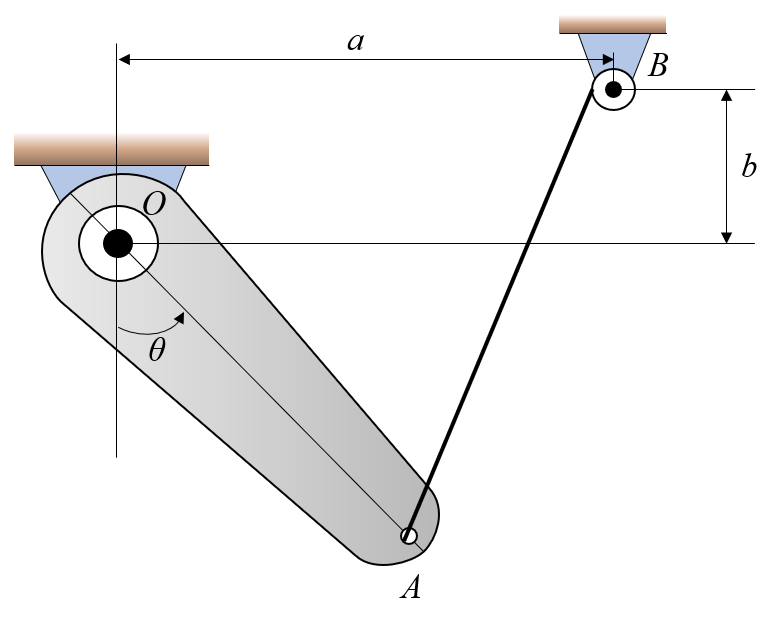
The arm OA can rotate freely around \(O\) and is actuated by the string attached in \(A\) and around \(B\). Let \(a=400\)mm, \(b=80\)mm and the length between \(O\) and \(A\) be \(r_{OA}=350\)mm. Furthermore let the center of graviy (COG) be located at \(120\)mm from \(O\) along the line \(OA\).
- Express the length \(|\mathbb{AB}|\) as a function of \(\theta\) and find the minimum distance and at which \(\theta\) this occurs for \(\theta\in[0,180^\circ]\).
- Find the above distance using an interactive visualization.
- How does the minimum vary with \(b\)?
Solution
Using the right-hand rule we define a coordinate system with \(x\) positively defined to the right, \(y\) positively defined up and thus \(z\) is given positively outward from the screen following the right-hand rule. See the figure below
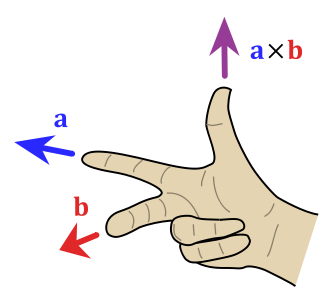
Even if the problem is simplified into two dimensions (2D problem or plane problem), we will still use three dimensions in our computations, to ensure that the cross product function can be utilized.
The point \(B\) is a fix point, it does not vary with \(\theta\), so it is easiest to describe: \[ \mathbb r_ {OB} = [400, 80, 0] \]
The center of mass \(\mathbb r_{OG}\) and \(\mathbb r_{OA}\) are both depending on \(\theta\) and have distances \(OA=350\) mm and \(OG=120\) mm, we start by defining the unit vector \(\mathbb e_{OA}\):
\[ \mathbb e_{OA} = [\sin\theta, -\cos\theta, 0]^T \]
Sanity check or test: Testing this is always a good idea, just set \(\theta\) to some angles for which the outcome is trivial. For, e.g., \(\theta=0\) we expect to get \(\mathbb e_{OA}=(\theta=0^\circ)=[0,-1,0]^T\), which indeed is the case. For \(\theta=90^\circ\) we expect to get \(\mathbb e_{OA}=(\theta=90^\circ)=[1,0,0]^T\), which is also is indeed the case.
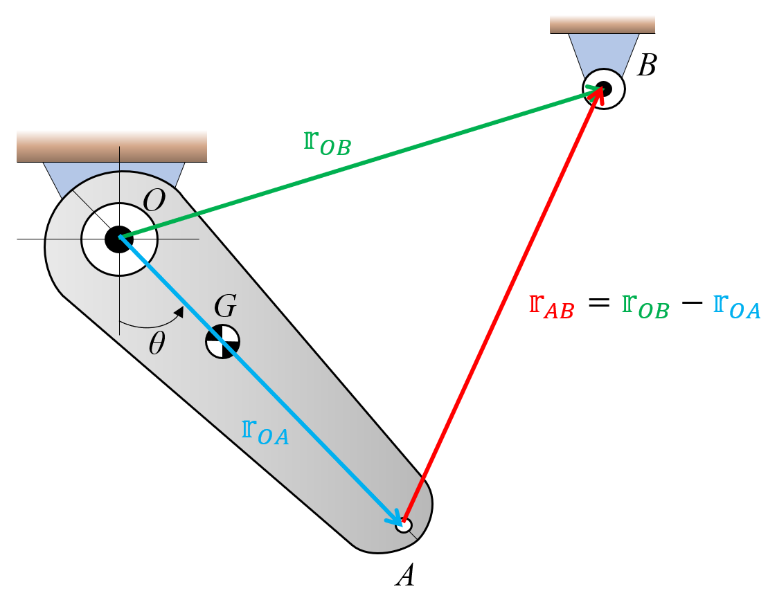
We define \(\mathbb r_{OG}=120\mathbb{e}_{OA}\) and \(\mathbb r_{OA}=350\mathbb {e}_{OA}\) and the vector \(\mathbb r_{AB}\) is given by the difference between \(\mathbb r_{OB}\) and \(\mathbb r_{OA}\):
\[ \mathbb r_{AB}=\mathbb r_{OB}-\mathbb r_{OA} \]
One can think of it as “head minus tail”, i.e., the head of \(\mathbb r_{AB}\) is in \(B\) and its tail in \(A\), see Figure 3.2.1.
The length is given by
\[ L(\theta) = AB = |\mathbb r_{AB}| = \sqrt{AB_x^2+AB_y^2} \]
The length, magnitude or norm is given by
r_AB = rr_AB.norm()This expression can now be plotted and we can easily see the solution
Show the code
import numpy as np
import matplotlib.pyplot as plt

# Convert r_AB into a numerical function using lambdi, but now using degrees
L_s_function = sp.lambdify(theta, r_AB.subs(theta, sp.rad(theta)), "numpy")

# Define a range of theta values in degrees (e.g., from 0 to 90)
theta_values_deg = np.linspace(0, 90, 90)

# Plot the function
plt.figure()
plt.plot(theta_values_deg, L_s_function(theta_values_deg),
         label=r'$r_{AB}(\theta)$', color='b')
plt.title(r'$r_{AB}(\theta)$', fontsize=14)
plt.xlabel(r'$\theta$ (degrees)', fontsize=12)
plt.ylabel(r'$r_{AB}$ (mm)', fontsize=12)
plt.grid(True)
plt.legend()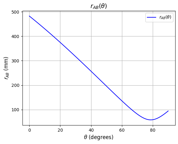
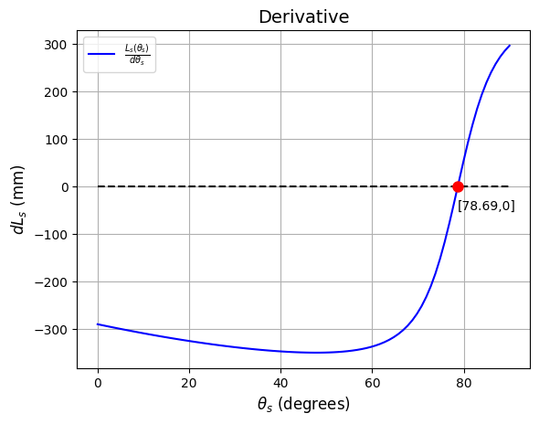
We can also compute the minimum point by solving the equation \(\frac{d}{d\theta}r_{AB}=0\)
dr_AB = sp.diff(r_AB, theta)dr_AB_fcn= sp.lambdify(theta, dr_AB.subs(theta, sp.rad(theta)), "numpy")theta_min = (sp.solve(dr_AB, theta)[0] * 180/sp.pi).evalf()Show the code
plt.figure()
plt.plot(theta_values_deg, dr_AB_fcn(theta_values_deg),
         label=r'$\frac{L_s(\theta_s)}{d\theta_s}$', color='b')
plt.plot([0,90],[0,0], color='k', linestyle='--')
plt.plot([theta_min],[0], 'o', markersize=8, color='red')
plt.text(theta_min, 0-50, f"[{theta_min:0.2f},0]")
plt.title("Derivative", fontsize=14)
plt.xlabel(r'$\theta_s$ (degrees)', fontsize=12)
plt.ylabel(r'$dL_s$ (mm)', fontsize=12)
plt.grid(True)
plt.legend()