Working in 3D is not too difficult once we get familiar with proper tools. Here we shall give a thorough walk-through of the process on a non-trivial example. The hardest part is the kinematics, i.e., describing the positions of the points relative to each other. Once this is done, formulating forces and moments to do equilibrium is a trivial matter with computer support.
3D Example application
We shall here learn to work with a rotated coordinate system.
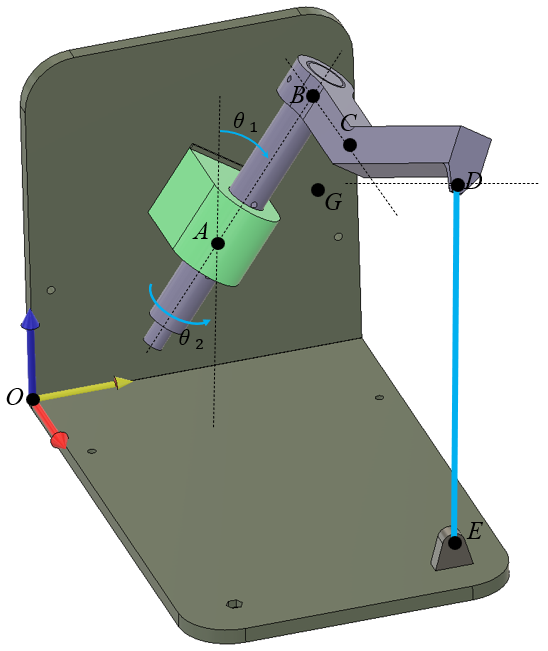
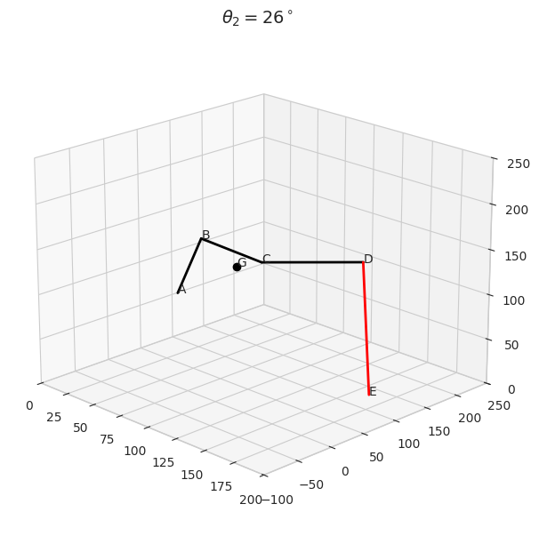
Figure 4.2.1: Kinematic figure
We start out by defining the coordinate system, the red axis is the x-axis, the green axis is the y-axis and the blue axis is the z-axis. See Figure 4.2.1.
\(A=(30, 60, 75)\) mm, \(r_{AB}=65\) mm, \(r_{BC}=50\) mm, \(\theta_1=35^\circ\) around the local \(x-\) axis at \(A\) and \(E=(145,40,0)\).
Let \(\theta_2\) denote the rotation of the shaft \(AB\). In the picture above, the \(\mathbb{r}_{BC}\) vector is parallel to the \(x-\) axis, and this is when \(\theta_2=0^\circ\).
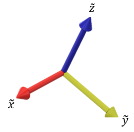
The center of gravity can be defined using local coordinates as: \(\mathbb r_{AG} = 34\tilde x + 51 \tilde z\), where \(\tilde x\) and \(\tilde z\) are the unit vectors in the local coordinate system according to Figure 4.2.2.:
Figure 4.2.2: Local coordinate system
Similarly, we can define \(\mathbb r_{CD}=70 \tilde x + 40 \tilde z\) using local coordinates.
Given the spring constant \(k=0.1\) N/mm and the unloaded spring length \(L_0=120\) mm:
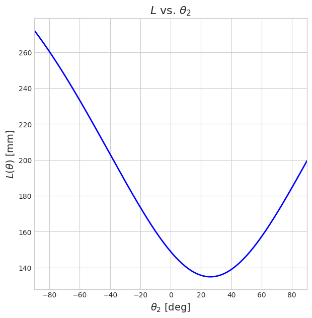
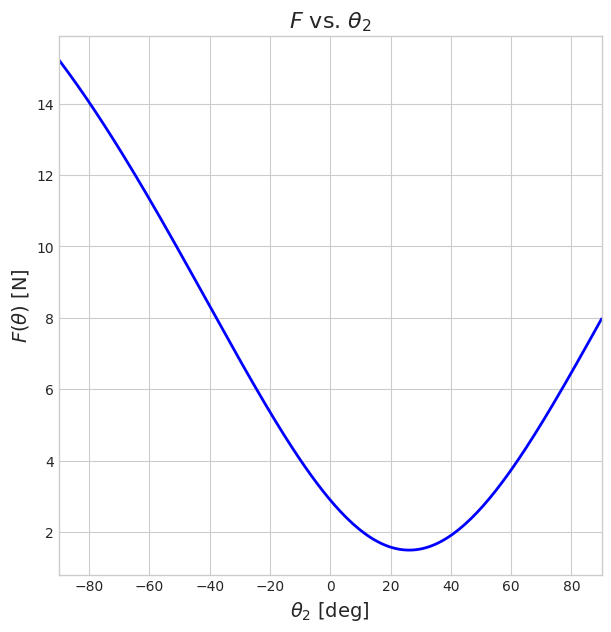
Determine and plot the length of the spring \(L_{DE}(\theta_2)\) as well as the spring force \(F(\theta_2)\).
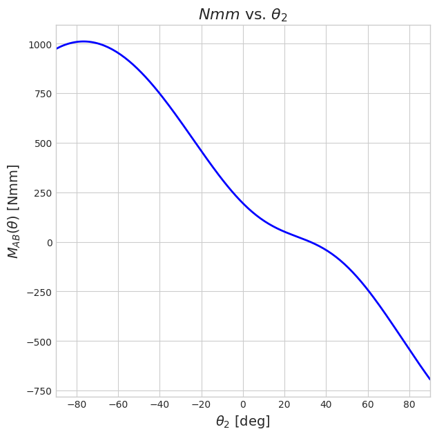
Determine and plot the moment which the motor needs to generate to rotate the shaft \(AB\), \(M_{AB}(\theta_2)\) for \(\theta_2 \in [90^\circ, -90^\circ]\)
Modeling - Kinematics
We are going to work with vectors to define the path from \(O\) to \(D\) and \(G\) as a function of the rotation angle \(\theta\). To do this, we need to introduce local coordinates and rotate these using rotation matrices:
We start by getting to point \(A\) using the vector \(\mathbb r_{OA}\). From here we need to establish the direction of the shaft axis, \(AB\), which we can do by rotating the \(\mathbb e_z\) vector around the \(x-\) axis by \(-\theta_1\) degrees (using the right hand rule).
This gives us our \(\mathbb e_{AB}\) direction vector:
Sympy has built in functions for rotation matrices. Note, however, that we need to use rot_ccw_axis1, rot_ccw_axis2 and rot_ccw_axis3 which adhere to the right-hand-rule convention! See sympy documentation for more information.
Note that we rotate \(-\theta_1\) due to the right hand rule, i.e., put the thumb in the direction of \(x\) and the fingers will point in the positive direction of rotation.
The shaft \(AB\) needs to rotate around its axis, or the \(\tilde{z}-\) axis. The rotation can be achieved by rotating around the global axis, \(x,y\) and \(z\). From the initial confguration, see below, where the shaft axis is aligned with the \(z\)-axis and \(\mathbb r_{BC}\) oriented towards the \(x-\) axis. To get the correct rotation of the shaft, we need to first rotate around the \(z-\) axis and then around the \(x-\) axis.
First we rotate around the \(z\) axis
Then we rotate around the \(x\) axis
Mathematically, this is the same as rotating our coordinate system by
Here, we get that the \(\tilde x\) -axis points in the positive \(y\) direction, the \(\tilde y\) -axis points in the negative \(x\) direction and the \(\tilde z\) -axis points in the positive \(z\) direction. This is correct, since we have rotated the coordinate system 90 degrees around the \(z\)-axis according to the right-hand-rule.
Now, we can also rotate around the \(x-\) axis by \(\theta_1 = -90^\circ\), we should get \(\tilde z = [0, 1, 0]^\mathsf T\)
We can confirm that the new coordinates point in the directions we expect. The \(\tilde x\) -axis points in the negative \(z\) direction, the \(\tilde y\) -axis points in the negative \(x\) direction and the \(\tilde z\) -axis points in the positive \(y\) direction. This is correct.
Thus have confirmed that the rotation makes sense, we have built confidence in our model and can set the rotation to solve our problem:
Zooming in at the force graph, we learn that the minimum force and length of the spring occurs at \(26^\circ\).
The maximum moment occurs at around \(-78^\circ\). The moment is zero around \(29.5^\circ\)
Rotating around a local axis
Another approach to rotating the coordinate system is to rotate around a local coordinate system. This makes the modeling and thinking easier. One does not need to be confined to thinking about rotations around global coordinates.
This can be done by rotating the \(z\) rotation matrix, \(\mathbb R_z\) around the \(x-\) axis by
This rotation matrix rotates vectors around the \(\tilde{z}\) axis. This approach still relies on defning the rotation matrix by rotating it around global axis. The order of rotations is important, thus chaining rotations can become tedious.
It would be nicer to have a function that lets us rotate around a arbitrary vector \(\boldsymbol u\). To achieve this we visit our favorite source of goodyness, Wikipedia, and find that the very elegant way of rotating a vector \(\boldsymbol v\) around an axis \(\boldsymbol u\) by an angle \(\theta\) according to the right-hand rule is stated as