7  Computer supported mechanics manifest

The first step in solving any mechanics problems is to start “by hand”, i.e. with a tablet or by using pen and paper. Draw a free body diagram, and define all relevant force vectors and positional vectors. Make sure that you understand the problem. State the equations of motion (Newton 2 and Euler 2) and compare the number of equations to the number of unknowns. The second step is to formulate the defined vectors and equations using a computer algebra system (CAS), then let a computer do all of the computations.

“It is unworthy of excellent men to lose hours like slaves in the labour of calculation which could safely be relegated to anyone else if machines were used.”

- Gottfried Wilhelm Leibniz in 1686

We are excellent, so we will use SymPy as our CAS!

7.1 SymPy

SymPy is a library for symbolic mathematics where the focus is on symbols rather than numbers. It allows you to manipulate and solve mathematical expressions symbolically, just like you would on paper. Numbers can still be used in SymPy, but they are not represented as numbers “under the hood”. In mechanics, the symbols we are dealing with are often unknown forces, moments, or positions. Think of the symbolic manipulation as everything we do before pluggin in numbers into our equations.

Import the sympy module only once at the beginning of your code. It is commonly imported as sp to reduce the amount of typing:

import sympy as sp

7.1.1 Variables and expressions

Symbolic (unknown) variables can now be defined:

x = sp.symbols('x')

Note that the x on the left hand side is a variable, and the 'x' on the right hand side is what will be shown as output. Use the same name for both, at least in the beginning until you have understood the difference.

It is good practice to state everything that is known about symbolic variables using “assumptions”:

x = sp.symbols('x', real=True, positive=True, integer=True)

Note that it must be lowercase “real” and nothing else, i.e. “Real” will just be ignored without any error messages. Multiple variables can be defined at the same time:

a, b = sp.symbols('a, b', real=True, positive=True)

Symbolic expressions can now be defined in terms of the symbolic variables:

f1 = sp.cos(x)**2 + sp.sin(x)**2
f1

\(\displaystyle \sin^{2}{\left(x \right)} + \cos^{2}{\left(x \right)}\)

If the last line of a cell is not an assignment (no equal sign), the contents of that variable/expression will be shown as output. If you prefer, you can use a semicolon ; to have multiple statements on the same line.

f2 = (a-b)**2; f2

\(\displaystyle \left(a - b\right)^{2}\)

Symbolic expressions can be expanded, factored, simplified and much more using for example:

f1.trigsimp()   # trigonometric simplification

\(\displaystyle 1\)

f2.expand()     # expands an expression

\(\displaystyle a^{2} - 2 a b + b^{2}\)

f1.simplify()   # general simplification (slower, but no thinking required)

\(\displaystyle 1\)

Any value like \(2, 3, \pi\) or \(\sqrt{2}\) can be substituted into a symbolic expression like this:

f2_eval = f2.subs(a, sp.pi).subs(b, sp.sqrt(2))
f2_eval

\(\displaystyle \left(\pi - \sqrt{2}\right)^{2}\)

To evaluate the above (exact) expression, we use evalf()

f2_eval.evalf()

\(\displaystyle 2.98383852477263\)

The number of decimals can be reduced by using round()

f2_eval.evalf().round(2)

\(\displaystyle 2.98\)

7.1.2 Vectors and systems of equations

To define a symbolic vector with a known magnitude \(||\mathbb{W}|| = mg\) and direction \(\mathbb{e}_W = [0, -1, 0]^\mathsf{T}\) the following vector definition can be used:

m, g = sp.symbols('m, g', real=True, positive=True)
WW = m * g * sp.Matrix([0, -1, 0]); WW

\(\displaystyle \left[\begin{matrix}0\\- g m\\0\end{matrix}\right]\)

Define another symbolic vector \(\mathbb{F}_A\) with unknown x- and y-components \(F_{Ax}\) and \(F_{Ay}\):

F_Ax, F_Ay = sp.symbols('F_Ax, F_Ay', real=True)
FFA = sp.Matrix([F_Ax, F_Ay, 0]); FFA

\(\displaystyle \left[\begin{matrix}F_{Ax}\\F_{Ay}\\0\end{matrix}\right]\)

Vectors can be added and subtracted just like you would expect. The sum of all forces:

N2 = WW + FFA; N2

\(\displaystyle \left[\begin{matrix}F_{Ax}\\F_{Ay} - g m\\0\end{matrix}\right]\)

To solve for the unknowns \(F_{Ax}, F_{Ay}\) and save them in a new dictionary named sol, we can use sp.solve():

sol = sp.solve([N2], [F_Ax, F_Ay])

Note the structure. We first specify the expression N2 as input, and then the unknown variables F_Ax and F_Ay as output. Multiple inputs can be given by comma-separation, just like the outputs. Note that N2 is not an equation in this example, but a sum of vectors, i.e. another vector. The sp.solve() function assumes that the right hand side of whatever we input is equal to zero if we do not tell it otherwise. To explicitly specify the right hand side as zero (the zero vector in this case), or something else, we have sp.Eq():

sol = sp.solve([sp.Eq(N2, sp.Matrix([0, 0, 0]))], [F_Ax, F_Ay])

The output from the two above cells are identical. The resulting values of \(F_{Ax}\) and \(F_{Ay}\) can now be accessed from the dictionary:

F_Ay_eval = sol[F_Ay]
F_Ay_eval

\(\displaystyle g m\)

Computing the vector/cross product \(\mathbb{F}_A\times\mathbb{W}\) is done using cross():

FFA.cross(WW)

\(\displaystyle \left[\begin{matrix}0\\0\\- F_{Ax} g m\end{matrix}\right]\)

Computing the scalar/dot product \(\mathbb{F}_A\cdot\mathbb{W}\) is done using dot():

FFA.dot(WW)

\(\displaystyle - F_{Ay} g m\)

Computing the norm \({F}_A = ||\mathbb{F}_A|| = \sqrt{\mathbb{F}_{Ax}^2 + \mathbb{F}_{Ay}^2 + \mathbb{F}_{Az}^2} = \sqrt{\mathbb{F}_A\cdot\mathbb{F}_A}\) can be achieved by using norm():

FFA.norm()

\(\displaystyle \sqrt{F_{Ax}^{2} + F_{Ay}^{2}}\)

Normalizing the length of a vector, i.e. computing the unit vector \(\mathbb{e}_{\mathbb{F}_{A}} = \frac{\mathbb{F}_A}{||\mathbb{F}_A||}\) is done using normalized():

FFA.normalized()

\(\displaystyle \left[\begin{matrix}\frac{F_{Ax}}{\sqrt{F_{Ax}^{2} + F_{Ay}^{2}}}\\\frac{F_{Ay}}{\sqrt{F_{Ax}^{2} + F_{Ay}^{2}}}\\0\end{matrix}\right]\)

Rotation matrices can be defined using sp.rot_axis1(), sp.rot_axis2() and sp.rot_axis3() like this:

theta = sp.symbols('theta', real=True)
Rx = sp.rot_axis1(theta) # x-axis rotation matrix
Ry = sp.rot_axis2(theta) # y-axis rotation matrix
Rz = sp.rot_axis3(theta) # z-axis rotation matrix
Rz

\(\displaystyle \left[\begin{matrix}\cos{\left(\theta \right)} & \sin{\left(\theta \right)} & 0\\- \sin{\left(\theta \right)} & \cos{\left(\theta \right)} & 0\\0 & 0 & 1\end{matrix}\right]\)

We can now for example rotate \(\mathbb{F}_A\) around the z-axis by matrix multiplication using the @-operator. Remember that rotational matrices are applied on the left side of a vector, and that multiple rotations can be chained (also from the left).

Rz @ FFA

\(\displaystyle \left[\begin{matrix}F_{Ax} \cos{\left(\theta \right)} + F_{Ay} \sin{\left(\theta \right)}\\- F_{Ax} \sin{\left(\theta \right)} + F_{Ay} \cos{\left(\theta \right)}\\0\end{matrix}\right]\)

Another operation that might come in handy is the scalar projection of \(\mathbb{A}\) along the direction of \(\mathbb{B}\). For this to work, \(\mathbb{B}\) must be normalized.

AA = 20 * sp.Matrix([sp.cos(sp.pi/2), sp.sin(sp.pi/2), 0]) # example vector
BB = sp.Matrix([sp.sqrt(2), sp.sqrt(3), 0]) # example vector

AA.dot(BB.normalized())

\(\displaystyle 4 \sqrt{15}\)

The vector projection of \(\mathbb{A}\) along the direction of \(\mathbb{B}\) can be computed using projection():

AA.project(BB)

\(\displaystyle \left[\begin{matrix}4 \sqrt{6}\\12\\0\end{matrix}\right]\)

7.2 NumPy

NumPy is a library for numerical calculations, where a floating point representation of numbers is used rather than symbols. It is a high-performance and heavy-duty calculator, optimized for modern computer hardware.

A common workflow is to perform algebra and/or equation solving on symbolic expressions using SymPy, and then to transition into a numerical representation using NumPy when it is time to perform calculations/plotting/etc.

Import the numpy module only once at the beginning of your code. It is commonly imported as np to reduce the amount of typing.

import numpy as np

We can convert symbolic expressions into numerical functions by using the sp.lambdify() function. The first input specifies the symbolic variables, and the second input specifies the symbolic expression that should be converted. As an example, consider the conversion of the rotation matrix Rx, which is a symbolic matrix containing the variable theta:

Rx_f = sp.lambdify([theta], Rx)

Rx_f is now a numerical function of theta which can be called directly with something like \(\pi/2\) radians to return a numerical rotation matrix:

Rx_np = Rx_f(np.pi/2)
Rx_np

array([[ 1.000000e+00,  0.000000e+00,  0.000000e+00],
       [ 0.000000e+00,  6.123234e-17,  1.000000e+00],
       [ 0.000000e+00, -1.000000e+00,  6.123234e-17]])

Note the usage of scientific notation, i.e. e+00 means to multiply by \(10^{00} = 1\) and e-17 means to multiply by \(10^{-17} \approx 0\).

Zero commonly gets represented like this in numerical calculations because of how computers work with floating point numbers.

As a second example consider the conversion of the symbolic vector WW, which contains two symbolic variables \(m\) and \(g\).

WW_f = sp.lambdify([m, g], WW)
WW_np = WW_f(20, 20).flatten()
WW_np

array([   0, -400,    0])

WW_np is now a numerical function of m and g.

Note also that the resulting numerical function WW_np should be flattened using flatten() to have the same behavior as the symbolic vector. This applies only to vectors, and not to matrices.

The numerical rotation matrix Rx_np can be multiplied by the numerical vector WW_np, where the output is also numerical. Remember that matrix multiplication should be performed using the @-operator:

Rx_np @ WW_np

array([ 0.0000000e+00, -2.4492936e-14,  4.0000000e+02])

Alternatively the numerical functions can be multiplied directly (do not forget to flatten):

Rx_f(np.pi/2) @ WW_f(20, 20).flatten()

array([ 0.0000000e+00, -2.4492936e-14,  4.0000000e+02])

Note that a sp.Matrix() object filled with numbers only (no unknowns/variables), can be converted directly into a numpy array (without sp.lambdify()) by the following operation:

WW_sym = WW.subs(m, 20).subs(g, 30) # symbolic vector
WW_np2 = np.array(WW_sym).astype(np.float64).flatten()
WW_np2

array([   0., -600.,    0.])

7.3 Matplotlib

Matplotlib is a data visualization library for creating static, animated and interactive figures. Pyplot is the interface that we use to conveniently access the library.

Import the Matplotlib module pyplot only once at the beginning of your code. It is commonly imported as plt to reduce the amount of typing.

import matplotlib.pyplot as plt

7.3.1 2D data plots

We begin by defining two new symbolic variables alpha and beta that will be used to define two new symbolic expressions V_x and V_y. The symbolic expressions are first converted into numerical functions using lambdify().

alpha, beta = sp.symbols('alpha, beta', real=True)
V_x = 10 * sp.cos(alpha)
V_y = beta * sp.sin(alpha)

V_x_np = sp.lambdify([alpha, beta], V_x)
V_y_np = sp.lambdify([alpha, beta], V_y)

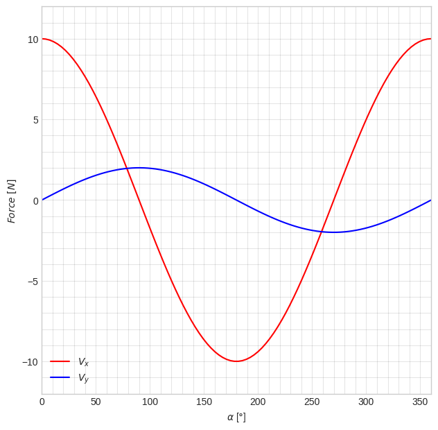
A very common thing we want to do is to plot how some function varies when we change its variables within some range. The following code is a minimal example of that.

It is good practice to separate “figure settings” from the actual drawing/plotting. Use comments # to separate code into individual sections in the same cell. We begin by setting the color-theme to seaborn-v0_8-whitegrid because it looks a bit nicer than the default. We initialize a new figure object fig with a specific size: 7.25 x 7.25 (inches). Then we add a new axis object ax to fig using the function add_subplot(). This is necessary to access some of the settings that we want to make, and it also enables us to plot multiple things in the same figure if we need to. The axis limits xlim and ylim are set manually, but can also be left out which will set them dynamically. The labels xlabel and ylabel are set to indicate what is shown on each axis. Do not forget to specify the units. Some parameters controlling the appearance of the background grid are modified using plt.grid() and plt.minorticks_on().

The actual data visualization happens with the two plt.plot() commands.

Note the creation of alphas using linspace() which contains \(100\) numbers between \(0\) and \(2\pi\).

It is good/best practice to always switch to degrees when you visualize, but always use radians when performing the actual calculations. Note how the first component of plt.plot() is simply multiplied by 180/np.pi to achieve this.

# 2D figure settings
plt.style.use('seaborn-v0_8-whitegrid')
fig = plt.figure(figsize=(7.25, 7.25))
ax = fig.add_subplot()
ax.set(xlim=[0.0, 360.0], ylim=[-12.0, 12.0], 
       xlabel=r'$\alpha$ [$\degree$]', ylabel=r'$Force~[N]$')
plt.grid(True, which='both', color='k', linestyle='-', alpha=0.1)
plt.minorticks_on()

# draw V_x and V_y for all alphas, with fixed beta=1 and beta=2
alphas = np.linspace(0, 2*np.pi, 100)
plt.plot(alphas*180/np.pi, V_x_np(alphas, 1), color='red', label=r'$V_x$')
plt.plot(alphas*180/np.pi, V_y_np(alphas, 2), color='blue', label=r'$V_y$')

# draw legend
plt.legend()

7.3.2 2D vector plots

We begin by defining some new numerical vectors that can be used for the following examples. They can easily be replaced by your own symbolic vectors using the methodology described in the SymPy and NumPy sections above:

theta = np.pi/3 # slider variable here for example!
rr_OA = 0.5 * np.array([np.cos(theta), np.sin(theta), 0])
rr_OB = 0.9 * np.array([np.sin(theta), np.cos(theta), 0])
rr_O = np.array([0, 0, 0])

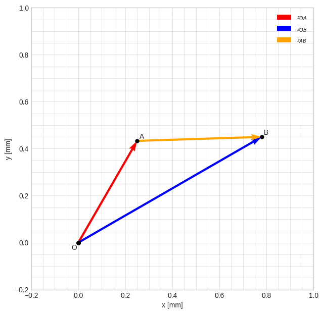
To verify that you have defined all positional vectors correctly, we typically want to visualize them. The following is a minimal 2D example of that.

The figure settings are the same as in the initial 2D data plot, with the addition of set_aspect() which forces the figure to have the same width as height. Drawing of vectors is done using quiver() and some points and text-labels are added using plot() and text(). Finally, a legend is added to the plot. Note the “slicing” of vectors in quiver(), for example: rr_O[:-1] where [:-1] means that the last entry (the z-component) of the initial 3D-vector is removed.

Note also that we have to set the scale-property of our quiver() for each set of xlim and ylim by trial-and-error. Note also the small adjustments to the position in the text() entries which prevents the text from being positioned exactly at each point. The zorder parameter sets the “layer” of the points, so that they are drawn on top of everything with a lower value than 10.

# 2D figure settings
plt.style.use('seaborn-v0_8-whitegrid')
fig2 = plt.figure(figsize=(7.25, 7.25))
ax2 = fig2.add_subplot()
ax2.set_aspect('equal')
ax2.set(xlim=[-0.2, 1.0], ylim=[-0.2, 1.0], xlabel='x [mm]', ylabel='y [mm]')
plt.grid(True, which='both', color='k', linestyle='-', alpha=0.1)
plt.minorticks_on()

# draw quivers
ax2.quiver(*rr_O[:-1], *rr_OA[:-1], 
           color='red', scale=1.2, label='$\\mathbb{r}_{OA}$')
ax2.quiver(*rr_O[:-1], *rr_OB[:-1], 
           color='blue', scale=1.2, label='$\\mathbb{r}_{OB}$')
ax2.quiver(*rr_OA[:-1], *(rr_OB[:-1]-rr_OA[:-1]),
           color='orange', scale=1.2, label='$\\mathbb{r}_{AB}$')

# if you dislike quiver(), you can draw lines using plot() and zip() instead
# ax2.plot(*zip(rr_O[:-1], rr_OA[:-1]), 
#          color='red', linewidth=2.5, label='$\\mathbb{r}_{OA}$')
# ax2.plot(*zip(rr_O[:-1], rr_OB[:-1]), 
#          color='blue', linewidth=2.5, label='$\\mathbb{r}_{OB}$')
# ax2.plot(*zip(rr_OB[:-1], rr_OA[:-1]), 
#          color='orange', linewidth=2.5, label='$\\mathbb{r}_{AB}$')

# draw points
ax2.plot(*rr_O, marker='o', color='black', markersize=5, zorder=10)
ax2.plot(*rr_OA, marker='o', color='black', markersize=5, zorder=10)
ax2.plot(*rr_OB, marker='o', color='black', markersize=5, zorder=10)

# draw point labels
ax2.text(*rr_O[:-1]-0.03, 'O') # - small adjustment
ax2.text(*rr_OA[:-1]+0.01, 'A') # + small adjustment
ax2.text(*rr_OB[:-1]+0.01, 'B') # + small adjustment

# draw legend
ax2.legend()

7.3.3 3D vector plots

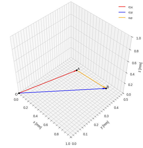
3D works in the same way as 2D, with the exception of the add_subplot() line that now also specifies the projection type as 3d. The view_init() command is used to rotate the camera view.

Note also that no slicing is required in 3D, since the vectors already have the correct “shape”. To make the arrow-heads look proportional in 3D, the parameter arrow_length_ratio is set manually, as the arrowhead size automatically scales up with the vector norm as well as the choice of xlim, ylim and zlim.

# 3D figure settings
plt.style.use('seaborn-v0_8-whitegrid')
fig3 = plt.figure(figsize=(7.25, 7.25))
ax3 = fig3.add_subplot(projection='3d')
ax3.view_init(elev=45, azim=-45)
ax3.set_proj_type('persp', focal_length=0.5) # or 'ortho' without focal_length
ax3.set_aspect('equal')
ax3.set(xlim=[0.0, 1.0], ylim=[0.0, 0.5], zlim=[0.0, 1.0], 
       xlabel='x [mm]', ylabel='y [mm]', zlabel='z [mm]')
plt.minorticks_on()

# draw quivers
ax3.quiver(*rr_O, *rr_OA, linewidth=1.5, 
           color='red', arrow_length_ratio=0.05, label='$\\mathbb{r}_{OA}$')
ax3.quiver(*rr_O, *rr_OB, linewidth=1.5, 
           color='blue', arrow_length_ratio=0.04, label='$\\mathbb{r}_{OB}$')
ax3.quiver(*rr_OA, *(rr_OB-rr_OA), linewidth=1.5, 
           color='orange', arrow_length_ratio=0.09, label='$\\mathbb{r}_{AB}$')

# # if you dislike quiver(), you can draw lines using plot() and zip() instead
# ax3.plot(*zip(rr_O, rr_OA), 
#          color='red', linewidth=2.5, label='$\\mathbb{r}_{OA}$')
# ax3.plot(*zip(rr_O, rr_OB), 
#          color='blue', linewidth=2.5, label='$\\mathbb{r}_{OB}$')
# ax3.plot(*zip(rr_OB, rr_OA), 
#          color='orange', linewidth=2.5,label='$\\mathbb{r}_{AB}$')

# draw points
ax3.plot(*rr_O, marker='o', color='black', markersize=4, zorder=9)
ax3.plot(*rr_OA, marker='o', color='black', markersize=4, zorder=9)
ax3.plot(*rr_OB, marker='o', color='black', markersize=4, zorder=9)

# draw point labels
ax3.text(*rr_O-0.025, 'O', fontsize=10, color='black', zorder=10)
ax3.text(*rr_OA+0.005, 'A', fontsize=10, color='black', zorder=10)
ax3.text(*rr_OB+0.005, 'B', fontsize=10, color='black', zorder=10)

# draw legend
ax3.legend()

7.4 Marimo

Marimo is a reactive notebook that you are hopefully using already to try out this code. It is reactive in the sense that if you change the value of a variable in one cell, all other cells with a reference to it will react. To fully utilize the power this gives you, interactive elements like buttons, sliders, switches, dropdown menus etc. can be added to your notebook. In mechanics, this lets you investigate the behavior of your models in a much more convenient way, without writing much code.

To enable interactive elements in the notebook, import marimo as mo only once at the beginning of your code:

import marimo as mo

7.4.1 Sliders

An interactive slider sl can be used to automatically update the value of any variable. Add the following code to its own cell, preferably right after creating a figure:

sl = mo.ui.slider(full_width=True, steps=np.linspace(0,2*np.pi,1000)); sl

This value of the slider can then be accessed via:

theta = sl.value

The variable theta can now be used as input to any numerical function, vector or matrix, and changing the slider will automatically re-evaluate all related calculations and/or plots.

If you want the slider to only update its value once when you release the mouse button instead of continuously, you can pass debounce=True as an argument to mo.ui.slider(). After clicking the slider once, left- and right- keyboard buttons can still be held down to update the value continously.

7.4.2 Switches

A switch sw can be used to toggle something on/off etc. Add the following code in a new cell:

sw = mo.ui.switch(label='Divine intellect'); sw

To access the state of the switch, we use sw.value which will be False as default, and True once toggled. Example usage could be for example toggling the legend on/off in a plot:

if sw.value: 
    ax2.legend() # draw a legend
else:
    pass # do nothing

7.4.3 Markdown

To access the value of a variable in a markdown-cell, you can use the following:

mo.md(rf"$$ \mathbb R_{{x}} = {sp.latex(Rx)}$$") # display Rx...
mo.md(rf"{rr_OA[0]:0.2f}") # display rr_OA[0] rounded to two decimals