Code
import sympy as sp                                       # Symbolical math tools
import numpy as np                                       # Numerical math tools
import matplotlib.pyplot as plt # Visualization toolsDetermine how all of the forces in the system varies as the direction of the 4000 N force changes. 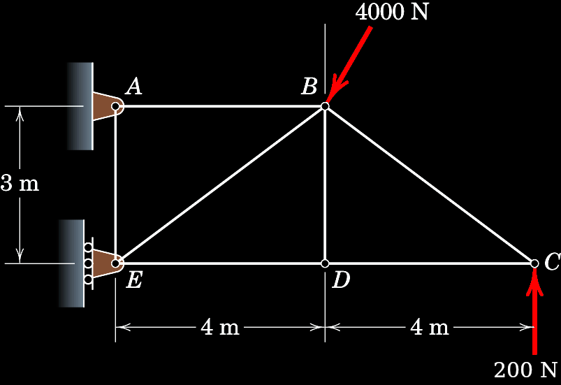
This is an example of the minimal amount of “paperwork” necessary before you start working with Python.
A free body diagram consists of several definitions: a coordinate system, points of interest, forces, moments and distances. Additionally, clearly define any known constants or other parameters that are allowed to vary. Finally, define all force- and positional vectors in terms of both knowns and unknowns. 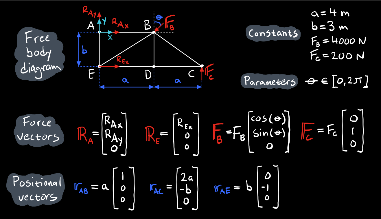
Compare the number of unknown variables to the number of equations you can establish for the given problem. If they are the same, you can proceed to coding. If not, more thinking and/or paperwork is required! 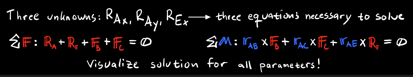
Imports
import sympy as sp # Symbolical math tools
import numpy as np # Numerical math tools
import matplotlib.pyplot as plt # Visualization toolsConstants
a = 4                                                    # [m] Distance ED
b = 3                                                    # [m] Distance AE
F_B = 4000                                               # [N] Force magnitude: B
F_C = 200                                                # [N] Force magnitude: C
Parameters
theta = sp.symbols('theta', real=True) # [rad] Angle at BVariables
R_Ax, R_Ay, R_Ex = sp.symbols('R_Ax, R_Ay, R_Ex', real=True) # [N] UnknownsForce vectors
RR_A = sp.Matrix([R_Ax, R_Ay, 0])                        # [N] Reaction force A
FF_B = F_B * sp.Matrix([sp.cos(theta), sp.sin(theta), 0])# [N] External force B
RR_E = sp.Matrix([R_Ex, 0, 0])                           # [N] Reaction force E
FF_C = F_C * sp.Matrix([0, 1, 0])                        # [N] External force C
Positional vectors
rr_AB = a * sp.Matrix([1, 0, 0])                         # [m] Vector from A-B
rr_AC = sp.Matrix([2*a, -b, 0])                          # [m] Vector from A-C
rr_AE = b * sp.Matrix([0, -1, 0])                        # [m] Vector from A-E
Newton’s second law
N2 = sp.Eq(RR_A + FF_B + RR_E + FF_C,
           sp.Matrix([0, 0, 0]))
N2
\(\displaystyle \left[\begin{matrix}R_{Ax} + R_{Ex} + 4000 \cos{\left(\theta \right)}\\R_{Ay} + 4000 \sin{\left(\theta \right)} + 200\\0\end{matrix}\right] = \left[\begin{matrix}0\\0\\0\end{matrix}\right]\)
Euler’s second law
E2 = sp.Eq(rr_AB.cross(FF_B) + rr_AC.cross(FF_C) + rr_AE.cross(RR_E),
           sp.Matrix([0, 0, 0]))
E2
\(\displaystyle \left[\begin{matrix}0\\0\\3 R_{Ex} + 16000 \sin{\left(\theta \right)} + 1600\end{matrix}\right] = \left[\begin{matrix}0\\0\\0\end{matrix}\right]\)
Solve for unknown variables
sol = sp.solve([N2, E2], [R_Ax, R_Ay, R_Ex])Symbolic -> Numerical
R_Ax_f = sp.lambdify([theta], sol[R_Ax])
R_Ay_f = sp.lambdify([theta], sol[R_Ay])
R_Ex_f = sp.lambdify([theta], sol[R_Ex])
Visualization
# figure settings
plt.style.use('dark_background')
fig = plt.figure(figsize=(8.00, 6.00))
ax = fig.add_subplot()
ax.set(xlabel='Angle θ [°]', ylabel='Reaction force [N]')
plt.grid(True, which='both', color='w', linestyle='-', alpha=0.1)
plt.minorticks_on()

# draw values
thetas = np.linspace(0, 2*np.pi, 100)
ax.plot(thetas*180/np.pi, R_Ax_f(thetas), 'red')
ax.plot(thetas*180/np.pi, R_Ay_f(thetas), 'green')
ax.plot(thetas*180/np.pi, R_Ex_f(thetas), 'blue')

# draw legend
ax.legend(['$R_{Ax}$', '$R_{Ay}$', '$R_{Ex}$'])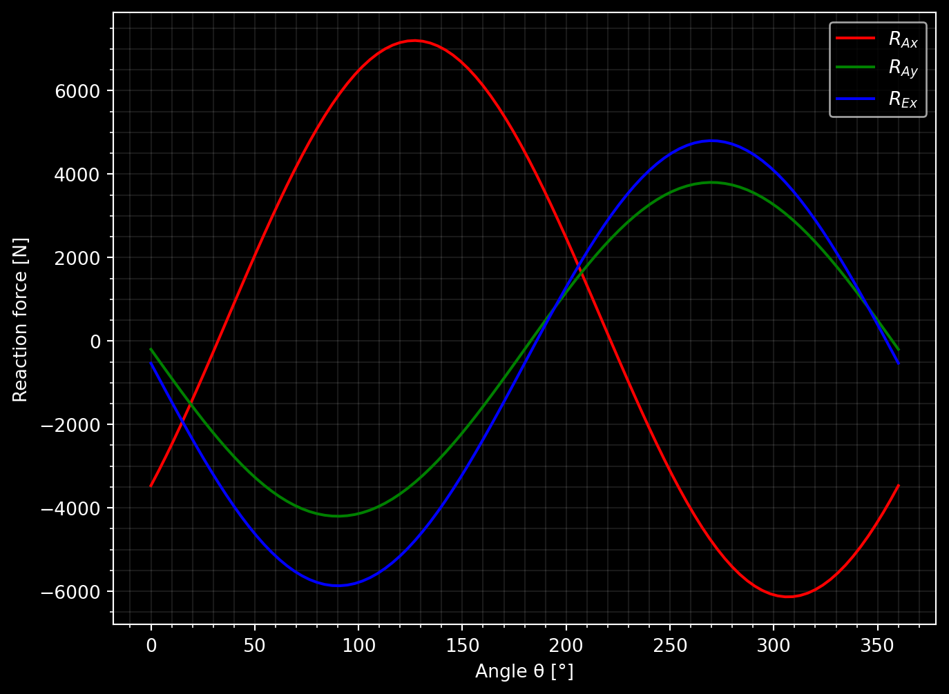
The beam is supported at A with rotational joints and a wire at B. The beam has a mass of \(m=475\) kg. There is also a force acting on the hook as shown in the figure.
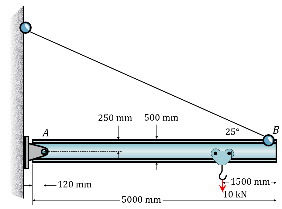
We start by selecting a point for our moments to be calculated around. In this case we select the center of the leftmost end of the beam and call that point O.
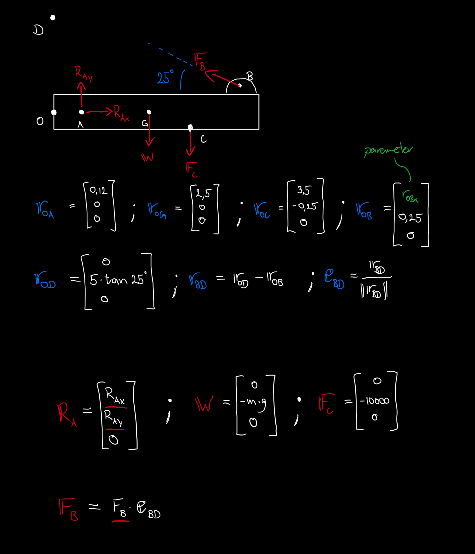
Then we create the necessary vectors between different points and how they relate to each other. We also name the points according the the figure below.
We can then define our force vectors and formulate our equations of equilibrium.
Constants
### Input
g = 9.81 # [m/s^2]
m = 475 # [kg]
We model the placement of B with a symbolic parameter \(r_{OBx}\) and then procede to create the vectors from O to the points of interest according to the figure.
\[ \mathbb{r}_{OB} = \begin{bmatrix} r_{OBx}\\ 0.25\\ 0 \end{bmatrix} \]
The y-coordinate of D can be calculated with
\[ r_{ODy} = 5\tan 25^\circ \]
r_OBx = sp.symbols("r_OBx", real=True, positive=True)

rr_OA = sp.Matrix([0.12, 0, 0])
rr_OG = sp.Matrix([2.5, 0, 0])
rr_OC = sp.Matrix([3.5, -0.25, 0])
rr_OB = sp.Matrix([r_OBx, 0.25, 0])

r_ODy = np.tan(25*np.pi/180)*5
rr_OD = sp.Matrix([0, r_ODy, 0])
The direciton for the wire and thus the wire force, \(\mathbb{F}_B\), can be calculated in the following way: \[ \mathbb{r}_{BD} = \mathbb{r}_{OD} - \mathbb{r}_{OB} \]
and
\[ \mathbb{e}_{BD} = \frac{\mathbb{r}_{BD}}{||\mathbb{r}_{BD}||} \]
# Direction of the wire force
rr_BD = rr_OD - rr_OB
ee_BD = rr_BD.normalized()
When it comes to the forces, we define the force vectors using the definitions from the free body diagram created earlier. We create symbolic variables for the unknown scalar values \(R_{Ax}\), \(R_{Ay}\), and \(F_B\).
### Define the force vectors
R_Ax, R_Ay, F_B = sp.symbols("R_Ax, R_Ay, F_B", real=True)
RR_A = sp.Matrix([R_Ax, R_Ay, 0])
WW = m*g*sp.Matrix([0, -1, 0])
FF_C = sp.Matrix([0, -10000, 0])
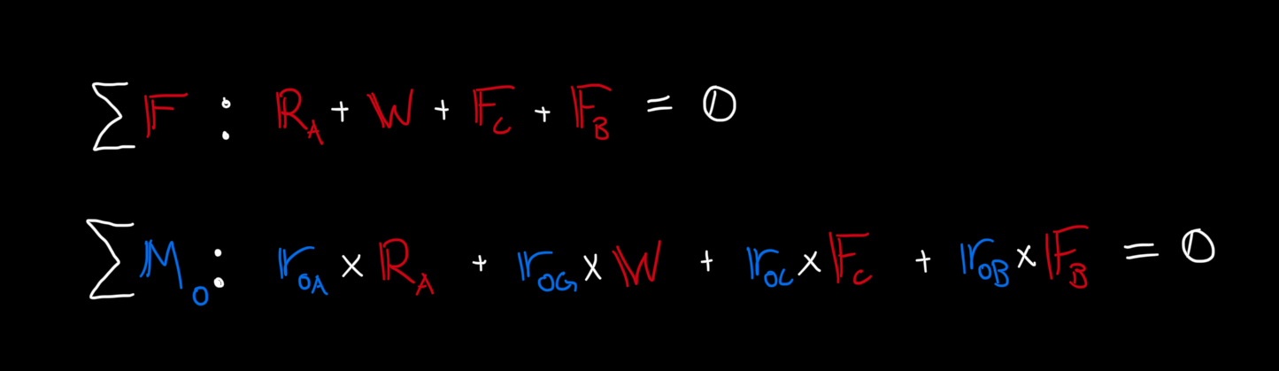
FF_B = F_B * ee_BDWe then establish the equations of equilibrium in the following way:
\[ \Sigma \mathbb{F}=\mathbb{0} : \mathbb{R}_A + \mathbb{W} + \mathbb{F}_C + \mathbb{F}_B = \mathbb{0} \]
\[ \Sigma \mathbb{M}=\mathbb{0}: (\mathbb{r}_{OA} \times \mathbb{R}_A) + (\mathbb{r}_{OG} \times \mathbb{W}) + (\mathbb{r}_{OC} \times \mathbb{F}_C) + (\mathbb{r}_{OB} \times \mathbb{F}_B) = \mathbb{0} \]
### Establish the equations of equlibrium and solve the system

sumF = sp.Eq(RR_A+WW+FF_C+FF_B,sp.Matrix([0,0,0]))
sumM = sp.Eq(rr_OA.cross(RR_A)+rr_OG.cross(WW)+rr_OC.cross(FF_C)+rr_OB.cross(FF_B),sp.Matrix([0,0,0]))

sol = sp.solve([sumF,sumM], [R_Ax, R_Ay, F_B])Finally, we plot the reaction forces as functions of \(r_{OBx}\).
### Plotting the reaction forces

# Create a plot and make settings
plt.style.use('seaborn-v0_8-whitegrid')
fig = plt.figure(figsize=(7, 7))
ax = fig.add_subplot()
ax.set(xlim=[0, 5], ylim=[-20000, 75000], xlabel='Placement of B [m]', ylabel='Force [N]')
ax.set_title("Reaction forces as a function to the wire placement")
plt.grid(True, which='both', color='k', linestyle='-', alpha=0.1)
plt.minorticks_on()

# Create the numerical data and functions
r_OBx_np = np.linspace(0,5,100)
F_B_f = sp.lambdify([r_OBx], sol[F_B], 'numpy')
R_Ax_f = sp.lambdify([r_OBx], sol[R_Ax], 'numpy')
R_Ay_f = sp.lambdify([r_OBx], sol[R_Ay], 'numpy')

# Creating each plot
ax.plot(r_OBx_np, F_B_f(r_OBx_np), linestyle='-', color='black', label="$F_{B}$")
ax.plot(r_OBx_np, R_Ax_f(r_OBx_np), linestyle='-', color='blue', label="$R_{Ax}$")
ax.plot(r_OBx_np, R_Ay_f(r_OBx_np), linestyle='-', color='red', label="$R_{Ay}$")


ax.legend()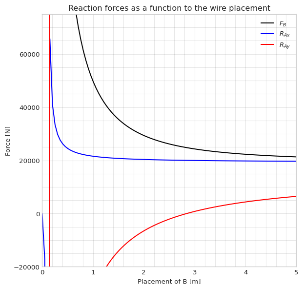
It is interesting to note what happens to the reaction forces when the placement is close to the point A. When the \(\mathbb{F}_B\) vector intercects A the reaction forces are infinite. Also \(\mathbb{F}_B\) is negative when \(\mathbb{F}_B\) intercects between O and A. That is of course not physical behaviour of a wire.
And we can also plot the geometry and force vectors in order to judge if the directions are reasonable given the calculated values for \(r_{OBx}=5\).
### Plotting the vectors and points

# Create a plot and make settings
#plt.style.use('seaborn-v0_8-whitegrid')
fig2 = plt.figure(figsize=(6, 6))
ax2 = fig2.add_subplot()
ax2.set(xlim=[-1, 6], ylim=[-2, 5], xlabel='X [m]', ylabel='Y [m]')
ax2.set_title("Visualization of the beam and forces")
plt.grid(True, which='both', color='k', linestyle='-', alpha=0.1)
plt.minorticks_on()

rr_OB_np = rr_OB.subs(r_OBx, 5).evalf()
rr_OD_np = rr_OD.evalf()

# Plotting the beam
ax2.plot([0,0,5,5,0], [-0.25,0.25,0.25,-0.25,-0.25], linestyle='-', color='black')
ax2.plot(*zip(rr_OB.subs(r_OBx, 5)[:-1],rr_OD[:-1]), linestyle='--', color='black', zorder=0)


# Plotting the points and labels
rr_O = np.array([0, 0, 0])
offset = 0.05

ax2.plot(*zip(rr_O), 'ok', ms=5)
ax2.text(rr_O[0]-5*offset,rr_O[1]+offset,"O")

ax2.plot(*rr_OA[:-1], 'ok', ms=5)
ax2.text(rr_OA[0]+offset, rr_OA[1]+offset,"A")

ax2.plot(*rr_OB_np[:-1], 'ok', ms=5)
ax2.text(rr_OB_np[0]+offset, rr_OB_np[1]+offset,"B")

ax2.plot(*rr_OG[:-1], 'ok', ms=5)
ax2.text(rr_OG[0]+offset, rr_OG[1]+offset,"G")

ax2.plot(*rr_OC[:-1], 'ok', ms=5)
ax2.text(rr_OC[0]+offset, rr_OC[1]+offset,"C")

ax2.plot(*rr_OD[:-1], 'ok', ms=5)
ax2.text(rr_OD[0]+offset, rr_OD[1]+offset,"D")


# Create vectors with numeric values
rr_OA_np = np.array(rr_OA).astype(np.float64)
rr_OC_np = np.array(rr_OC).astype(np.float64)
rr_OG_np = np.array(rr_OG).astype(np.float64)
WW_np = np.array(WW).astype(np.float64)
FF_C_np = np.array(FF_C).astype(np.float64)
FF_B_np = np.array(FF_B.subs({r_OBx:5,F_B:F_B_f(5)})).astype(np.float64)
RR_A_np = np.array(RR_A.subs({R_Ax:R_Ax_f(5), R_Ay:R_Ay_f(5)})).astype(np.float64)

# Plotting the force vectors
ax2.quiver(*rr_OC_np[:-1], *FF_C_np[:-1], color='orange', scale=100000, label="$\\mathbb{F}_C$")
ax2.quiver(*rr_OB_np[:-1], *FF_B_np[:-1], color='red', scale=100000, label="$\\mathbb{F}_B$")
ax2.quiver(*rr_OA_np[:-1], *RR_A_np[:-1], color='red', scale=100000, label="$\\mathbb{R}_A$")
ax2.quiver(*rr_OG_np[:-1], *WW_np[:-1], color='blue', scale=50000, label="$\\mathbb{W}$")


ax2.legend()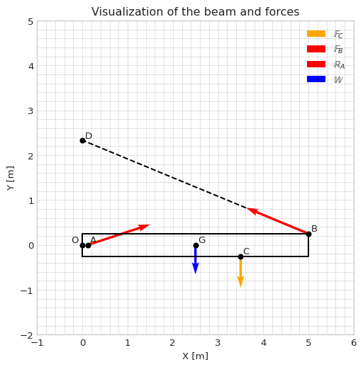
The structure shown in the figure is supported at A, B and C from the floor. The force acting on the point D represents a human with mass \(m=80\) kg.
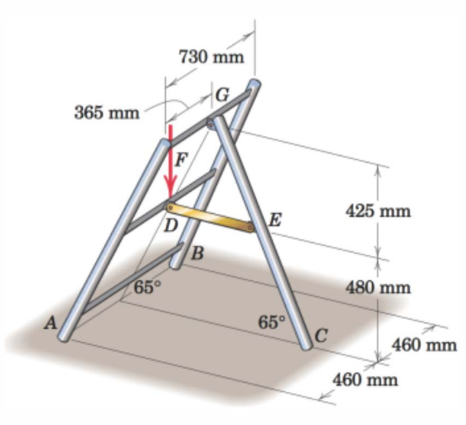
Before we begin the formal solution, we can reason about the problem and see if its possible to simplify it. In this case we note that the points D and G are placed in the center of the structure relative to A and B. Based on our intuition and previous knowledge of forces we see that it is reasonable to simplify this problem to 2D as the reaction force in A and B will be equal. The reaction force we would calculate for the point representing A and B will be the sum of the two.
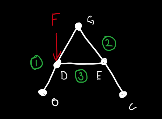
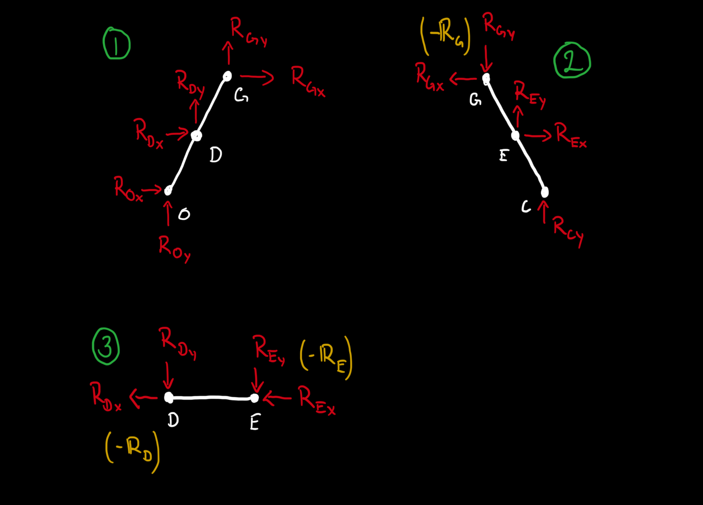
Based of this, we start by determining we need to create free body diagrams of the bodies ODG, CEG, and DE.
We select points for our moments to be calculated around. In this case we select the point O in the body ODG, point C in CEG, and point D in DE.
Then we create the necessary vectors between different points and how they relate to each other.
We can then define our force vectors and formulate our equations of equilibrium.
Constants
### Input
theta = 65 * sp.pi/180 #[rad]
m = 80 #[kg]
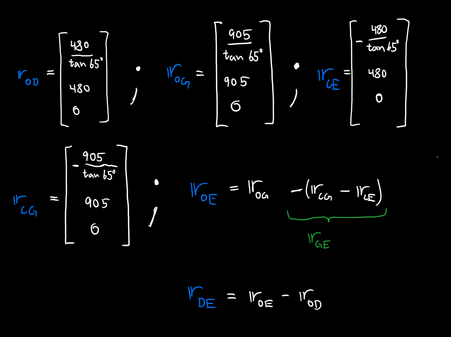
g = 9.82 #[m/s^2]Based on the free body diagrams and the decisions for what points to calculate moments around, we see the need for the following vectors: \(\mathbb{r}_{OD}\), \(\mathbb{r}_{OG}\), \(\mathbb{r}_{CE}\), \(\mathbb{r}_{CG}\), and \(\mathbb{r}_{DE}\).
The first elements in \(\mathbb{r}_{OD}\), \(\mathbb{r}_{OG}\), \(\mathbb{r}_{CE}\), and \(\mathbb{r}_{CG}\) can be calculated with for example:
\[ r_{ODx} = \frac{480}{\tan 65^\circ} \]
Because the structure is symmetric the first element in \(\mathbb{r}_{CE}\) will be, \(r_{CEx} = -\frac{480}{\tan 65^\circ}\)
### Define position vectors and vectors for moment calculations

rr_OD = sp.Matrix([480/sp.tan(theta), 480, 0])
rr_OG = sp.Matrix([905/sp.tan(theta), 905, 0])
rr_CE = sp.Matrix([-480/sp.tan(theta), 480, 0])
rr_CG = sp.Matrix([-905/sp.tan(theta), 905, 0])
To define \(\mathbb{r}_{DE}\) we can use the vectors already defined in the following way:
\[ \mathbb{r}_{OE} = \mathbb{r}_{OG} - (\mathbb{r}_{CG}-\mathbb{r}_{CE}) \]
and
\[ \mathbb{r}_{DE} = \mathbb{r}_{OE} - \mathbb{r}_{OD} \]
rr_OE = rr_OG - (rr_CG-rr_CE)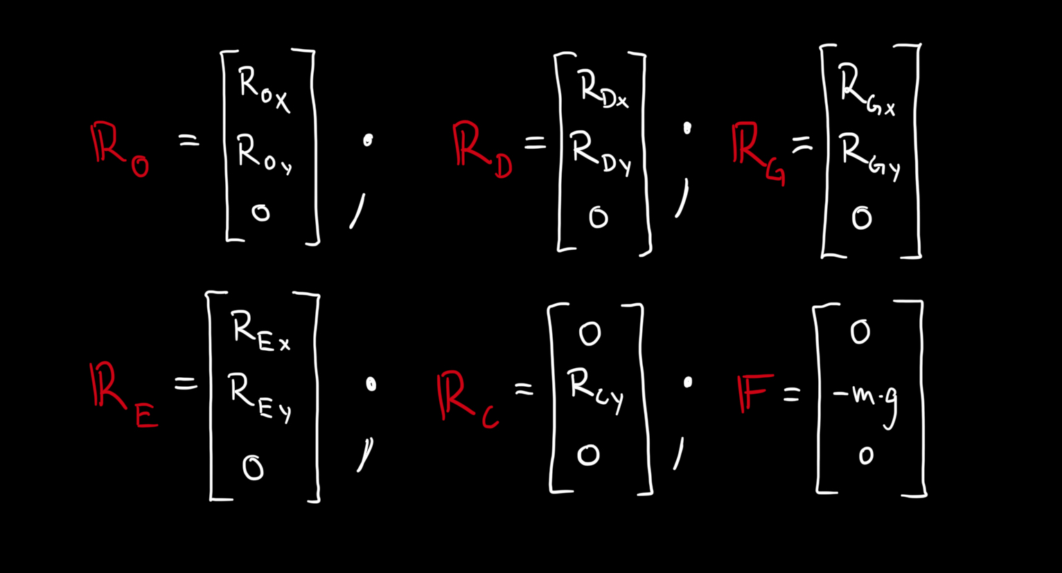
rr_DE = rr_OE - rr_ODWhen it comes to the forces, we define the force vectors using the definitions from the free body diagram created earlier. We create symbolic variables for the unknown scalar values.
### Define force vectors
R_Ox, R_Oy, R_Dx, R_Dy, R_Gx, R_Gy, R_Ex, R_Ey, R_Cy = sp.symbols(
'R_Ox, R_Oy, R_Dx, R_Dy, R_Gx, R_Gy, R_Ex, R_Ey, R_Cy', real=True)
RR_O = sp.Matrix([R_Ox, R_Oy, 0])
RR_D = sp.Matrix([R_Dx, R_Dy, 0])
RR_G = sp.Matrix([R_Gx, R_Gy, 0])
RR_E = sp.Matrix([R_Ex, R_Ey, 0])
RR_C = sp.Matrix([0, R_Cy, 0])
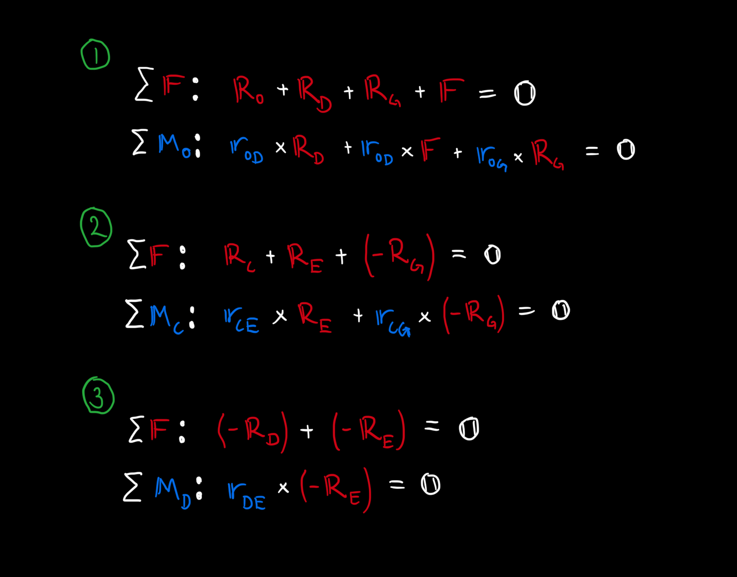
FF = sp.Matrix([0, -m*g, 0])We then establish the equations of equilibrium in the following way:
Body 1 (ODG)
\[ \Sigma \mathbb{F}: \mathbb{R}_O + \mathbb{R}_D + \mathbb{F} + \mathbb{R}_G = \mathbb{0} \]
\[ \Sigma \mathbb{M}_O: (\mathbb{r}_{OD} \times \mathbb{R}_D) + (\mathbb{r}_{OD} \times \mathbb{F}) + (\mathbb{r}_{OG} \times \mathbb{R}_G) = \mathbb{0} \]
Body 2 (CEG)
\[ \Sigma \mathbb{F}: \mathbb{R}_C + \mathbb{R}_E + (-\mathbb{R}_G) = \mathbb{0} \]
\[ \Sigma \mathbb{M}_C: (\mathbb{r}_{CE} \times \mathbb{R}_E) + (\mathbb{r}_{CG} \times (-\mathbb{R}_G)) = \mathbb{0} \]
Body 3 (DE)
\[ \Sigma \mathbb{F}: (-\mathbb{R}_D) + (-\mathbb{R}_E) = \mathbb{0} \]
\[ \Sigma \mathbb{M}_D: \mathbb{r}_{DE} \times (-\mathbb{R}_E) = \mathbb{0} \]
### Establish the equations of equlibrium and solve the system

# Equilibrium for body 1
sumF1 = sp.Eq(RR_O + RR_D + FF + RR_G, sp.Matrix([0,0,0]))
sumM1 = sp.Eq(rr_OD.cross(RR_D) + rr_OD.cross(FF) + rr_OG.cross(RR_G), sp.Matrix([0,0,0]))

# Equilibrium for body 2
sumF2 = sp.Eq(RR_C + RR_E + (-RR_G), sp.Matrix([0,0,0]))
sumM2 = sp.Eq(rr_CE.cross(RR_E) + rr_CG.cross(-RR_G), sp.Matrix([0,0,0]))

# Equilibrium for body 3
sumF3 = sp.Eq((-RR_D) + (-RR_E), sp.Matrix([0,0,0]))
sumM3 = sp.Eq(rr_DE.cross(-RR_E), sp.Matrix([0,0,0]))

# Solve the system of equations
sol = sp.solve([sumF1,sumM1,sumF2,sumM2,sumF3,sumM3],
[R_Ox, R_Oy, R_Dx, R_Dy, R_Gx, R_Gy, R_Ex, R_Ey, R_Cy])Our expectation based on intuition is that the reaction forces from the floor should be pointing up. That implies that \(R_{Oy}\) and \(R_{Cy}\) should be positive, which is what we observe. The larger part of the applied force \(\mathbb{F}\) is taken up at O, since D is closer to O than to C in the X-direction. Since we have no external force in the X-direction, we expect \(R_{Ox}=0\), which we also get in our calculations. From the negative value of \(R_{Ex}\) and positive value of \(R_{Dx}\) we can conclude from free body diagram 3 that the body DE is in tension.