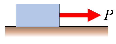
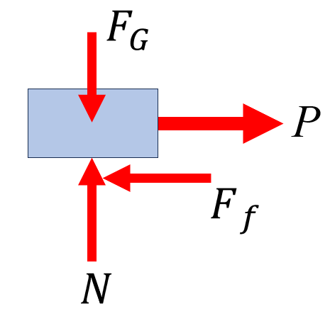
The box with the mass \(m\) kg is exposed to an external force \(P\) according to the left figure. Doing a free body diagram and applying Newton’s third law reveals a force \(F\) acting opposite to \(P\) along the contact surface. The magnitude of this friction force depends on the type of surface and the normal force \(N\). The relation between the normal force and friction force can be modelled using the Coulombs law:
\[
\boxed{ F \leq \mu_s N }
\]
where \(\mu_s\) is known as the static coefficient of friction. Coulomb developed a friction theory in the 1700 s for dry friction. This model assumes a linear relationship between \(F\) and \(N\) and even if we can empirically show that this does not generally hold for an arbitrarily large \(N\), Coulombs law is taken to be “good enough” for most situations, but should be used with care.
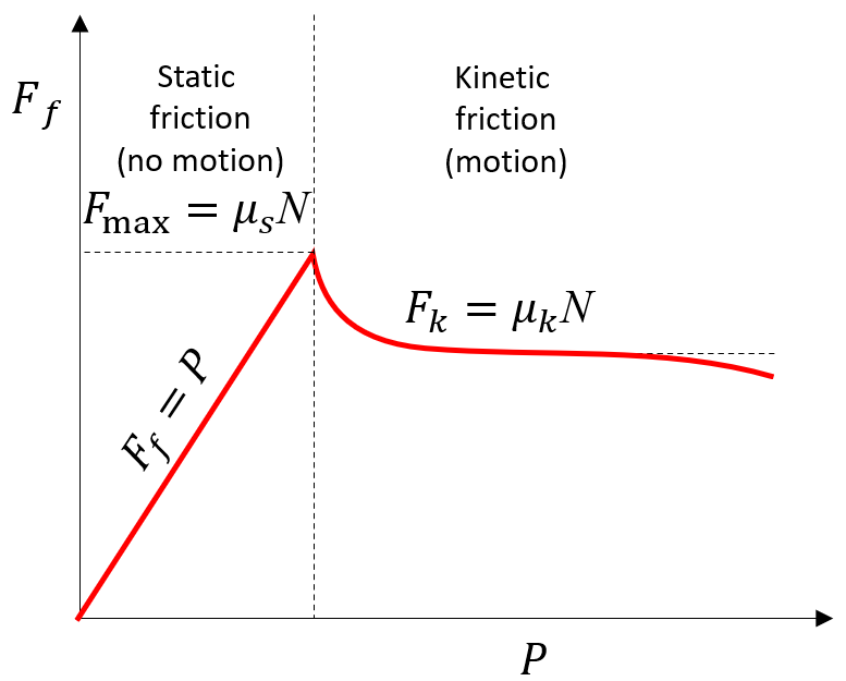
Figure 5.3.2: Relation between the external force \(P\) and friction force \(F_f\).
As the force \(P\) exceeds the largest possible frictional force \(F_{\max }\) the box will start to slide and get an acceleration, thus the model transitions to what is known as kinetic friction and the opposing force is given by \(F_k=\mu_k N\), where \(\mu_k\) is the kinetic coefficient of friction. This is where statics ends and dynamics continues.
The coefficients of friction can be calculated from empirical observations using measurements of forces, positions or angles.
⚠ Note
Any list containing the coefficient will be approximate, good accuracy is application dependent and must be measured.
Here is a list for (a rough) reference
Material
\(\mu_s\)
\(\mu_k\)
Steel on steel
\(0.1-0.3\)
\(0.03-0.3\)
Steel on wood
\(0.5-0.7\)
\(0.2-0.5\)
Leather on metal
\(0.3-0.6\)
\(0.2-0.3\)
Break pad on cast iron
0.4
0.3
Hemp rope on steel
0.3
0.2
Teflon on Teflon
0.05
0.05
Rubber on metal
\(0.4-0.5\)
\(0.3-0.4\)
Rubber on asphalt
\(0.7-1.0\)
\(0.5-0.8\)
Rubber on ice
0.1
0.05
⚠ Note
Note that Coulombs law is a very simple model in the world of tribology. Many applications need more sophisticated models of friction.
⚠ Note
For any problem involving rough surfaces where frictional forces need to be taken into account one needs to determine if the bodies are at rest or sliding. In general there are several types of states in contact points on a body. If we have a friction coefficient \(\mu_s\) and have the situation
\(F<\mu_s N\) then static equilibrium is possible since the surfaces can generate the needed friction force that is required for static friction.
\(F=\mu_s N\) then static equilibrium is still possible. This is a limit, often we write \(F_{\max }=\mu_s N\), to show that this is the maximum friction force, this limit is also known as fully established friction.
\(F>\mu_s N\) then static equilibrium is impossible. The surfaces cannot produce the frictional force that is required to keep static equilibrium. The body begins to slide, accelerates and we get dynamic equilibrium \(F=\mu_k N\), at this point the problem is transitioned into a dynamic problem and we have \(\Sigma F=m a\).
The basic rule for analysis with friction is that the frictional force-vector \(\mathbb F\) is set to be in the direction that opposes potential movement.
Essentially there two types of problem statements
All external forces except friction forces are known and we need to determine if the friction force can balance the external forces. This means that we need to check if \(F \leq \mu_s N\) in the contact surface, otherwise we have sliding and the problem is a dynamic problem with \(F=\mu_k N\).
Some external forces are unknown and we want to know how much more we can load the body until sliding occurs. This means that we add \(F_i=\mu_s N_i\) to all rough contact points and include these friction equations in the equilibrium equations. Solving for the unknown forces to answer the problem statement.
We show some typical examples involving friction.
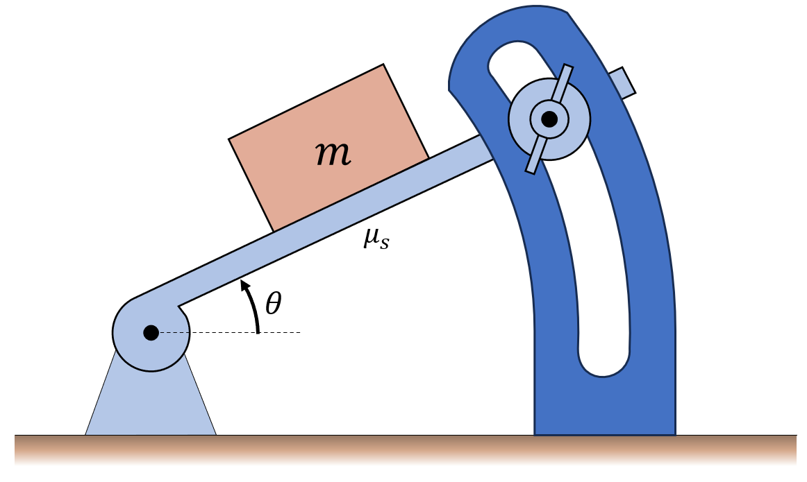
Example 1: A box on a slope
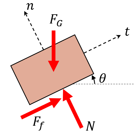
Determine the maximum angle \(\theta\) for which the box with mass \(m\) will not slide down the slope. The coefficient of static friction between the surfaces is \(\mu_s\).
Solution
FBD
Since we’re using a CAS, we can establish a normal coordinate system using the tangential direction \(t\) and the normal direction \(n\) to the slope. Once these directions are established we can easily express the force vectors in these directions and pose the equations of equilibrium.
We have equilibrium equations and an additional friction equation \(F_{\max }=\mu_s N\). Then we just solve for as many variables as we have equations.
The direction vector in the tangential direction is given by
$$ \left[\begin{matrix}F_{f} \cos{\left(\theta \right)} - N \sin{\left(\theta \right)}\\F_{f} \sin{\left(\theta \right)} + N \cos{\left(\theta \right)} - g m\\0\end{matrix}\right] = \left[\begin{matrix}0\\0\\0\end{matrix}\right] $$
Additionally we have the friction equation
ekv2 = sp.Eq(F_f, mu*N)
$$ F_{f} = N \mu $$
All together we have three equations and three unknowns. We can solve for the unknowns using SymPy.
sol = sp.solve([ekv1, ekv2], [F_f, N, mu], dict=True)[0]
$$
\begin{align*}
F_f = g m \sin{\left(\theta \right)} \\
N = g m \cos{\left(\theta \right)} \\
\mu = \tan{\left(\theta \right)}
\end{align*}
$$
Here we have that \(\theta = \tan^{-1}(\mu_s)\), also known as the angle of friction.
⚠ Note
A note for SymPy solve function. There are a number of ways solve returns solutions. For unique solutions we expect a list of one element containing a dict. Sometimes we just get the dict. One needs to check the output and use correct syntax to extract the solution.
In the above case we get a list with one element, which is a dict. First we need to index into the list and grab index 0 then we have the dict.
Note also that we explicitly use dict=True to get a dict as output. This should be the default behaviour of SymPy. But not always. In this case for unknown reasons, if omitted, we would get a list of solutions instead and not a dict.
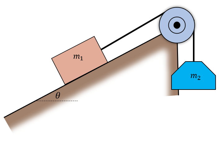
Two masses are rigged according to the figure. In what interval does \(m_2\) need to be in to prevent sliding of \(m_1\). Let \(\mu_s=0.3\) and \(\theta=20^{\circ}\).
Solution - Reformulation of the problem
We need to ensure that we understand the problem. This is imperitive to solve any engineering problem correctly. If in doubt, ask the problem owner for a clarification.
Let’s break down the above problem statement:
We \(m_2\) need to find the interval of \(m_2\) such that \(m_1\) does not slide. This means that we need to find the maximum and minimum values of \(m_2\) such that \(m_1\) is in static equilibrium. In other words:
Find
\[
m_{2, \min} < m_2 < m_{2, \max}
\]
such that \(m_1\) is in static equilibrium.
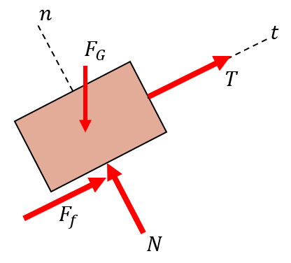
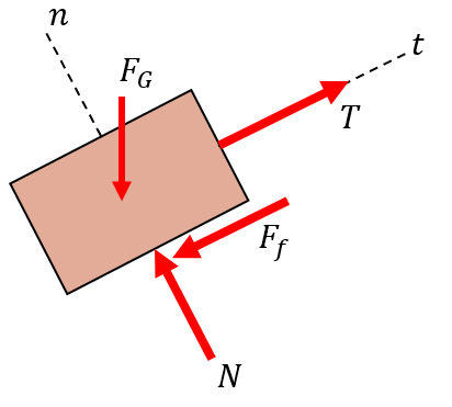
This gives rise to two cases: depending on if the box is just about to start gliding up or down. These cases result in two FBDs where the direction of the friction force is opposing the direction of movement.
Case 1: \(m_1\) is just about to start sliding down, i.e., finding \(m_{2\min}\)
An assumption we make is that the force \(T\) is transmitted through the pulley without any losses. This means that the tension in the rope is constant. We can also assume that the mass of the rope is negligible. This means that the tension in the rope is constant and equal to \(m_2 g\).
Kinematics
We need to establish the directions \(t\) and \(n\). Starting with the tangential direction \(t\) we have
\[
\mathbb e_t = [\cos \theta, \sin \theta, 0]^\mathsf T
\] The normal direction is given by \[
\mathbb e_n = [\cos \theta + 90^\circ, \sin \theta + 90^\circ, 0]^\mathsf T
\]
For a verification of the directions, see Section 13.2.2.
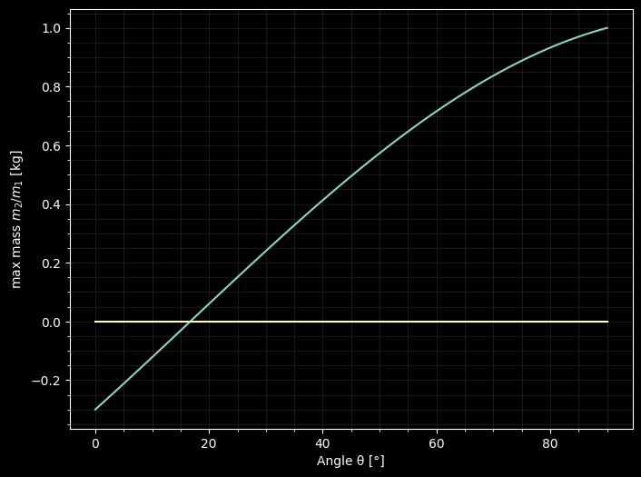
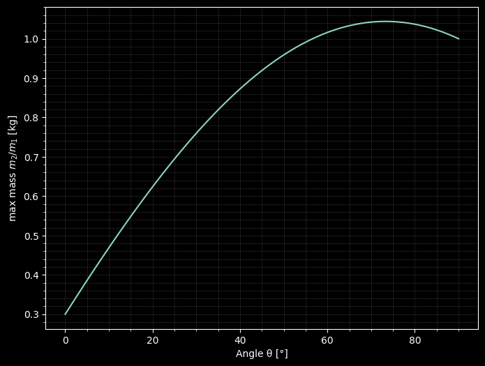
Feasibility analysis: At close to \(90^{\circ}\) the frictional force is so small that we get \(m_1=m_2\). At zero degrees the model does not work since we would get negative masses. Case 1 does not exists below slopes of ca \(17^{\circ}\), i.e., the box cannot slide downwards if the slope is less than \(17^{\circ}\).
Case 2: \(m_1\) is just about to start sliding up, i.e., finding \(m_{2\max}\)
In this case we have the following forces, with the friction force being reversed
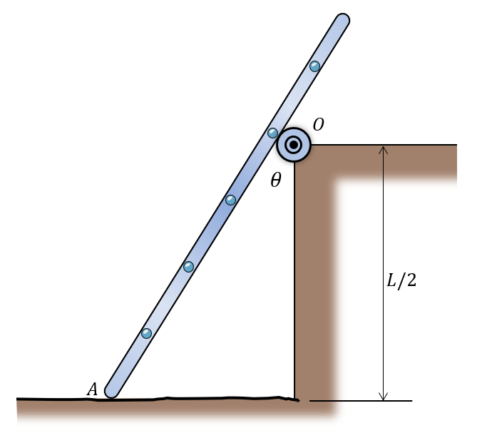
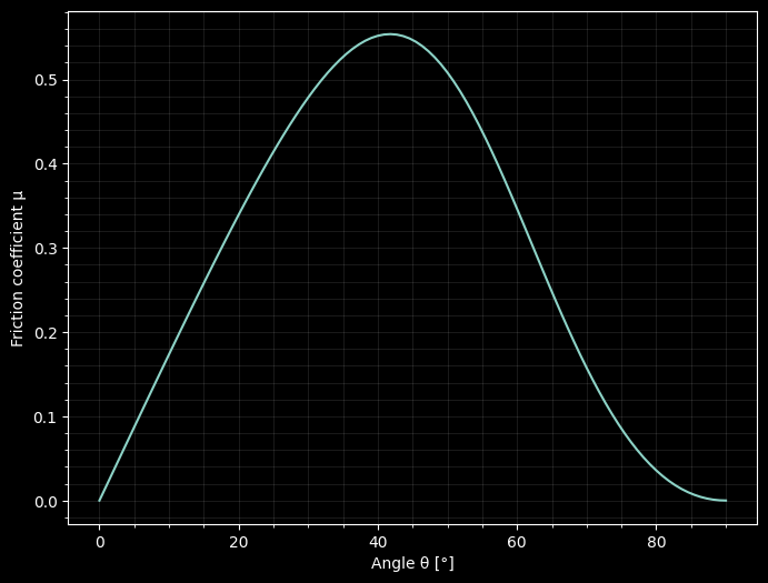
Determine the least possible \(\mu_s(\theta)\) at \(A\) such that the homogenous rod with a mass of \(m\) does not slide. There is no friction at \(O\). Disregard the radius of the roller at O. Draw a graph of \(\mu_s(\theta)\) for valid angles.
Solution
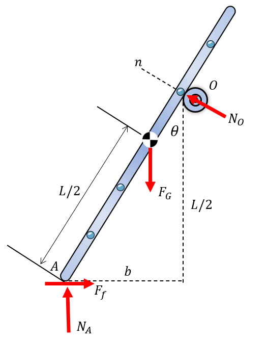
FBD
We start by defining the kinematics, the position of \(A\) needs to be defined as a function of that angle \(\theta\). Using trigonometry we recognize the triangle and have
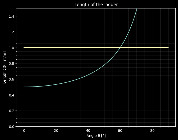
As seen from the ladder length graph, we cannot go beyond \(60^\circ\). This can also be verified usinga sketch in CAD
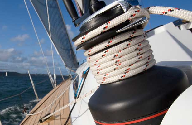
Example 4 - Flexible belts (Capstan equation)
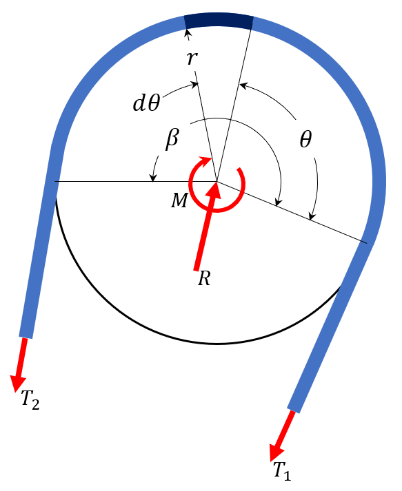
Ropes and belts which are wrapped around cylinders are a very common application for static friction in mechanics. We shall look closer at the problem.
Free body diagram
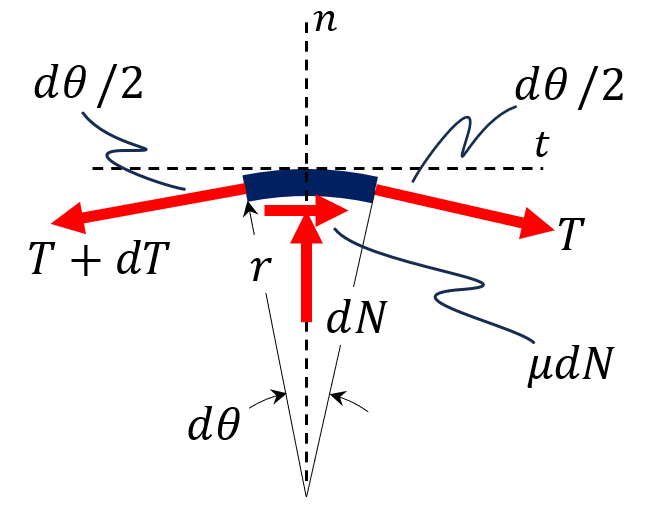
Infinitesimal belt element
Figure 5.3.6: Flexible belt free body diagram
A rope is wrapped some angle \(\beta \in[0, \infty]\) radians around a cylinder. We cut a small piece \(d \theta\) at an arbitrary angle \(\theta \in[0, \infty]\) and create a FBD according to the figure. We are interested in the maximum force and examine the limit just before sliding. The force equilibrium is divided into a tangential \((t)\) and radial \((n)\) direction
Since both dT and \(d \theta\) are very small, their product is even smaller and can be neglected, i.e., \(dTd \theta \ll dT, d \theta\)
Thus we end up with
\[
\left\{\begin{array}{l}
\mu dN=dT \\
dN=T d \theta
\end{array}\right.
\]
Eliminating \(dN\) and moving things around we can formulate a simple ordinary differential equation
\[
\frac{dT_2}{d \theta}=\mu T_2
\]
with the boundary condition \(T_2(0)=T_1\)
For which we can easily get the solution using SymPy symbolic differential equation solver dsolve:
import sympy as spfrom sympy import difftheta, mu, T1 = sp.symbols('theta, mu, T1', real=True)# Here we define the function T2T2 = sp.Function('T2')T2(theta)
\(\displaystyle T_{2}{\left(\theta \right)}\)
# Define the Differential EquationDE = sp.Eq(diff(T2(theta), theta), mu * T2(theta))DE
Ok, so with, e.g., \(\mu_s=0.25\) (hamp against steel according to some table) and wrapped five times we get
from sympy import exp, pimu =0.25T2 = T1 * exp(mu*5*2*pi)T2.evalf(6)
\(\displaystyle 2575.97 T_{1}\)
We see that the force \(T_2\) needs to be over 2500 times larger than \(T_1\) to be in balance. The Capstan equation (5.3.1) is extremely useful in many applications, e.g., belt breaking, winches, cranes, gearboxes, etc.
For a cool application see this video by Aaed Musa: