import sympy as sp                                       # Symbolical math tools
import numpy as np                                       # Numerical math tools
import marimo as mo                                      # Interactivity tools
import matplotlib.pyplot as plt # Visualization tools6.1 Forward kinematics
Problem
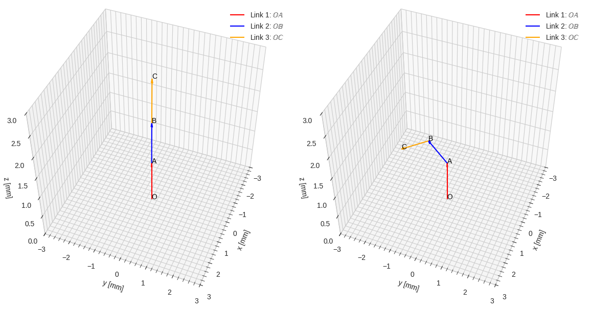
Determine the (x,y,z) position of the end effector (C) in a three-linked robotic arm. In the initial configuration (left figure), the O-joint can rotate around the Z-axis, while the A an B joints can rotate around the X-axes.
Solve the problem by using reference frames for the links OA, OB and OC.

Code
We begin with the usual stuff, importing the tools that we will use later.
Joint angles
The final position of the end effector is a function of the three joint angles alpha_O, alpha_A and alpha_B, which we know will be real-valued.
alpha_O, alpha_A, alpha_B = sp.symbols('alpha_O, alpha_A, alpha_B', real=True)Local link vectors
The links of the robot are described using the three local vectors OA_loc, AB_loc and BC_loc, before any rotation has been applied. The OA, AB and BC segments are of unit length in this example, and are oriented along +Z in their own individual reference frames.
OA_loc = 1 * sp.Matrix([0, 0, 1]) # oriented along +Z in its own reference frame
AB_loc = 1 * sp.Matrix([0, 0, 1]) # oriented along +Z in its own reference frame
BC_loc = 1 * sp.Matrix([0, 0, 1]) # oriented along +Z in its own reference frame
Reference frame: O
Introduce a new fixed and global reference frame O_r. In cartesian coordinates, this is simply the identity matrix where each column represents a basis vector, i.e. \(\mathbb{i}=[1, 0, 0]^\mathsf{T}\), \(\mathbb{j}=[0, 1, 0]^\mathsf{T}\) and \(\mathbb{k}=[0, 0, 1]^\mathsf{T}\).
O_r = sp.eye(3)Reference frame: OA
The first joint at O will now be rotated. The new reference frame OA_r is defined by computing O_r @ sp.rot_ccw_axis3(alpha_O) where sp.rot_ccw_axis3() is a rotation matrix counter-clockwise around Z. Depending on the motor configuration of the robot, we use the corresponding rotation matrix \(\mathbb{R}_x\), \(\mathbb{R}_y\) or \(\mathbb{R}_z\).
The local link vector OA_loc is then transformed into the global link vector OA by using the reference frame and the matrix multiplication: OA_r @ OA_loc
OA_r = O_r @ sp.rot_ccw_axis3(alpha_O) # rotate OA_r alpha_O radians around axis3
OA = OA_r @ OA_loc                 # local link vector -> global link vector
Reference frame: AB
The second joint rotation is handeled in the same way. The only difference being that we now base this operation on the already rotated OA_r. The global link vector is once again retrieved by multiplication with the reference frame.
AB_r = OA_r @ sp.rot_ccw_axis1(alpha_A) # rotate OA_r alpha_A radians around axis1
AB = AB_r @ AB_loc                  # local link vector -> global link vector
Reference frame: BC
The third and final rotation works exactly the same, and builds on the previously rotated reference frame AB_r. The “pattern” for adding even more links than three should now be obvious.
BC_r = AB_r @ sp.rot_ccw_axis1(alpha_B) # rotate B_r alpha_B radians around axis1
BC = BC_r @ BC_loc                  # local link vector -> global link vector
Symbolic end effector
To compute the end effector position (or any other position of interest on the robot for that matter), just add the global link vectors together.
OA + AB + BC\(\displaystyle \left[\begin{matrix}\sin{\left(\alpha_{A} \right)} \sin{\left(\alpha_{O} \right)} \cos{\left(\alpha_{B} \right)} + \sin{\left(\alpha_{A} \right)} \sin{\left(\alpha_{O} \right)} + \sin{\left(\alpha_{B} \right)} \sin{\left(\alpha_{O} \right)} \cos{\left(\alpha_{A} \right)}\\- \sin{\left(\alpha_{A} \right)} \cos{\left(\alpha_{B} \right)} \cos{\left(\alpha_{O} \right)} - \sin{\left(\alpha_{A} \right)} \cos{\left(\alpha_{O} \right)} - \sin{\left(\alpha_{B} \right)} \cos{\left(\alpha_{A} \right)} \cos{\left(\alpha_{O} \right)}\\- \sin{\left(\alpha_{A} \right)} \sin{\left(\alpha_{B} \right)} + \cos{\left(\alpha_{A} \right)} \cos{\left(\alpha_{B} \right)} + \cos{\left(\alpha_{A} \right)} + 1\end{matrix}\right]\)
Numerical end effector
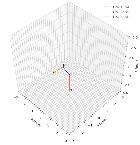
Evaluating the numerical coordinates for the set of joint angles \(\alpha_O = 0°\), \(\alpha_A = 45°\), \(\alpha_B = 45°\) we get:
angles = {alpha_O: 0*sp.pi/180, alpha_A: 45*sp.pi/180, alpha_B: 45*sp.pi/180}
OA_np = np.array(OA.subs(angles).evalf()).astype(np.float64).flatten()
AB_np = np.array(AB.subs(angles).evalf()).astype(np.float64).flatten()
BC_np = np.array(BC.subs(angles).evalf()).astype(np.float64).flatten()

OA_np + AB_np + BC_np
array([ 0. , -1.70710678, 1.70710678])Verification
To verify that everything really works as expected we should create a visualization.
# 3D figure settings
plt.style.use('seaborn-v0_8-whitegrid')
fig = plt.figure(figsize=(7.25, 7.25))
ax = fig.add_subplot(projection='3d')
ax.view_init(elev=45, azim=-45)
ax.set_proj_type('persp', focal_length=0.5) # or 'ortho' without focal_length
ax.set_aspect('equal')
ax.set(xlim=[-3.0, 3.0], ylim=[-3.0, 3.0], zlim=[0, 3.0],
       xlabel='x [mm]', ylabel='y [mm]', zlabel='z [mm]')
plt.minorticks_on()

# draw quivers
ax.quiver(*[0, 0, 0], *OA_np, linewidth=1.5,
           color='red', arrow_length_ratio=0.1, label='Link 1: $\\mathbb{OA}$')
ax.quiver(*OA_np, *AB_np, linewidth=1.5,
           color='blue', arrow_length_ratio=0.1, label='Link 2: $\\mathbb{OB}$')
ax.quiver(*(OA_np+AB_np), *BC_np, linewidth=1.5,
           color='orange', arrow_length_ratio=0.1, label='Link 3: $\\mathbb{OC}$')

# draw point labels
ax.text(*[0, 0, 0], 'O', fontsize=10, color='black', zorder=10)
ax.text(*OA_np+0.005, 'A', fontsize=10, color='black', zorder=10)
ax.text(*OA_np+AB_np+0.005, 'B', fontsize=10, color='black', zorder=10)
ax.text(*OA_np+AB_np+BC_np+0.005, 'C', fontsize=10, color='black', zorder=10)

# draw legend
ax.legend()
In the marimo notebook, we could also add a slider for each joint angle and play around with it until we have convinced ourselves that everything is working correctly.