If a body has an insignificant rotation compared to the path its center of gravity travels, it is said to be a particle. In later chapters we will make an proper introduction to generalized Newtonian-Euler motion equations, but for now, suffice to say if either the rotational acceleration or the size of the body is small enough, then we can neglect the change of angular momentum
The equation of motion for a particle is given by Newton’s second law:
\[
\sum F = m a
\]
and the rotational equation of motion is given by Euler’s second law:
\[
\sum M_G = \bar{I}\alpha
\]
If either the angular acceleration, \(\alpha\) or the size of the body (and thus \(\bar I\)) is small enough, then we can neglect the change of angular momentum, and the rotational equation of motion reduces to:
Figure 6.2.1: The flywheel must be treated as a rigid body; it is being accelerated and de-accelerated, thus it generates a rotational moment around its axis, by design, providing an energy reservoir to the system.
Figure 6.2.2: This marble can be treated as a particle since it rotational speed does not significantly influences its path.
Preliminaries
We start with kinematics and the mathematical descriptions of a bodies position, velocity and acceleration. This is the foundation of dynamics, including kinetics.
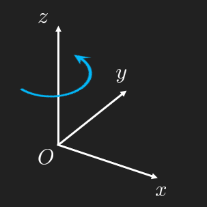
Assume an universal coordinate system and stick to it! We can choose between cartesian, normal and polar coordinate systems.
Coordinate system
Vector notation
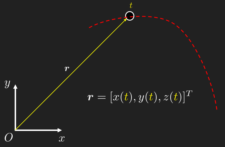
Position Vector
The position of a bodies center of gravity as a function of time \(t\) can be expressed using the position vector \(\mathbb{r}(t) = [x(t), y(t), z(t)]^T\) where each component is a function of the same independent variable \(t\). The components are called coordinate functions and \(\mathbb{r}(t)\) is known as the parameter curve with the parameter \(t\). The parameter curve is also known as the curve or path.
Velocity
Velocity Vector
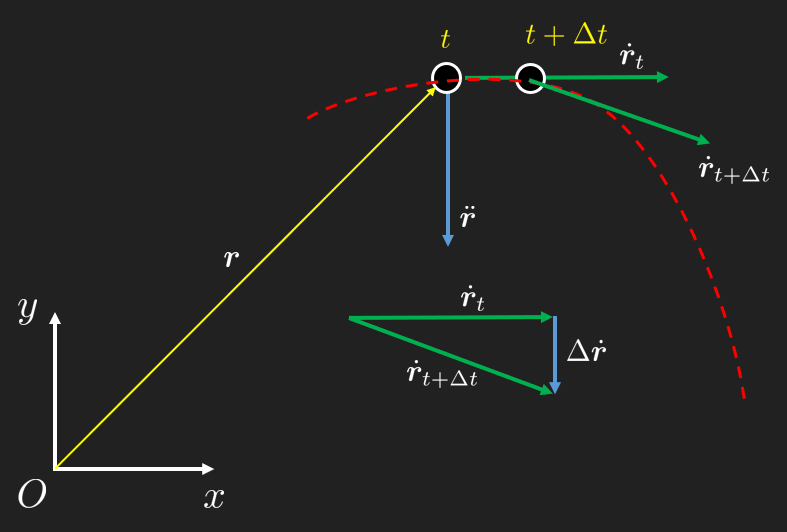
The mean velocity between two positions \(\mathbb{r}(t)\) and \(\mathbb{r}(t+\Delta t)\) can be described as \(\bar{\mathbb{v}} = \frac{\Delta \mathbb{r}}{\Delta t}\). In the limit where \(\Delta t \to 0\) we get the time derivate of the position vector, known as the velocity vector
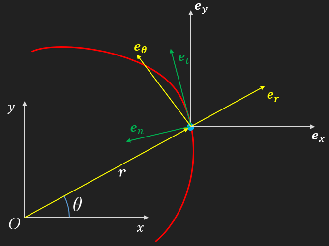
As can be seen in the animation, the velocity vector \(\dot{\mathbb{r}}\) at \(t\) is always tangential to the path.
The dot notation in \(\dot{r}\) or in \(\dot{\ddot{\ddot{\ddot{\ddot{r}}}}} = \frac{d^9}{dt^9}r\) (a.k.a. Newton’s abomination) comes from Newton who studied dynamic problems and needed to develop the mathematics to deal with these problems.
The mathematics came to be known as calculus which was expanded and is really made up by a great many contributors (Leibnitz, Lagrange). see e.g., this video for an historical overview.
The magnitude of the velocity vector, \(|\dot{\mathbb{r}}|\), is known as the speed. The difference between velocity and speed being that velocity also contains information about the direction of the object.
Acceleration
Similarly, the acceleration is given by the change of velocity over time, \(\frac{d\dot{\mathbb{r}}}{dt}\). The average acceleration at time \(t\) can be formulated as
From the animation we can see that the acceleration is pointing inwards, towards the center of curvature. Also, we see that the acceleration in general differs from the direction of the position vector. The acceleration vector can be decomposed into a tangential and a normal component, \(\mathbb{a} = a_t \mathbb{e}_t + a_n \mathbb{e}_n\) where \(\mathbb{e}_t\) is the unit tangent vector and \(\mathbb{e}_n\) is the unit normal vector. The tangential component \(a_t\) is responsible for changes in speed, while the normal component \(a_n\) is responsible for changes in direction. If the speed is constant, then \(a_t = 0\) and the acceleration is purely normal.
Acceleration Animation
Rectilinear motion
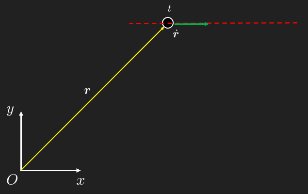
In the special case of rectilinear motion (motion without curvature), such as described in Figure 6.2.3
Figure 6.2.3: Rectilinear Motion
the position vector reduces to a single component, for example \(x(t)\), and the velocity and acceleration reduces to the time derivatives of this single component. We sometimes use the (simple) scalar notation
\[
s = |\mathbb{r}|=x(t), v = |\dot{\mathbb{r}}|=\dot x(t) \text{ and } a = |\ddot{\mathbb{r}}|=\ddot x(t)
\tag{6.2.4}\]
We can express these scalar values using the Leibniz notation for time derivative
\[
v = \frac{ds}{dt} \text{ and } a = \frac{dv}{dt}
\tag{6.2.5}\]
solving for the time increment \(dt\), we get
\[
dt = \frac{ds}{v} = \frac{dv}{a}
\tag{6.2.6}\]
from which we get
\[
\boxed{a \, ds = v \, dv}
\tag{6.2.7}\]
Which is convenient to use in special cases where we are not interested in time explicitly, but should be used with care and really be avoided all together, instead the proposed working method is described in what follows.
Differential equations
Working purely with the scalar notation from the previous section is troublesome. A strong recommendation is to avoid the use of derived formulas often found in classical books in mechanics and formularies, since it is often more tedious to figure out the assumptions under which these formulas are valid than to create a model using the differential equations directly. Many ready-to-go formulas assume the acceleration to be constant. We shall also refrain from using the notations \(s\), \(v\) and \(a\) for varying position, velocity and acceleration since it is harder to let go of the “thinking by formularies” and move towards “Concept Based Modeling” with “Computational Thinking”. Instead use \(\mathbb{r}, \dot{\mathbb{r}}\) and \(\ddot{\mathbb{r}}\) along with knowledge of differential equations!
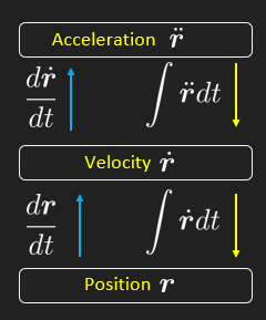
Remember that the derivative and integral operator works naturally on vectors i.e.,
The velocity (vector) is the time derivative of the position (vector), \(\dot{\mathbb{r}} = \frac{d\mathbb{r}}{dt}\) with respect to time, \(t\). The magnitude \(|\dot{\mathbb{r}}|\) is known as speed (scalar value). The direction is tangent to the trajectory path. The acceleration (vector) is the time derivative of the velocity (vector) \(\ddot{\mathbb{r}} = \frac{d\dot{\mathbb{r}}}{dt} = \frac{d}{dt}(\frac{d\mathbb{r}}{dt}) = \frac{d^2\mathbb{r}}{dt^2}\), or the second time derivative of the position (vector).
The acceleration (vector) is the time derivative of the velocity (vector) \(\ddot{\mathbb{r}} = \frac{d\dot{\mathbb{r}}}{dt} = \frac{d}{dt}(\frac{d\mathbb{r}}{dt}) = \frac{d^2\mathbb{r}}{dt^2}\), or the second time derivative of the position (vector).
In what follows we shall rely more on working with the vector form of \(\mathbb{r}\) and formulate the differentials as ordinary differential equations which we can easy solve using either a symbolic differential equation solve, e.g., sympy.dsolve() or numerically by utilizing e.g., the Euler method.
The recommended way
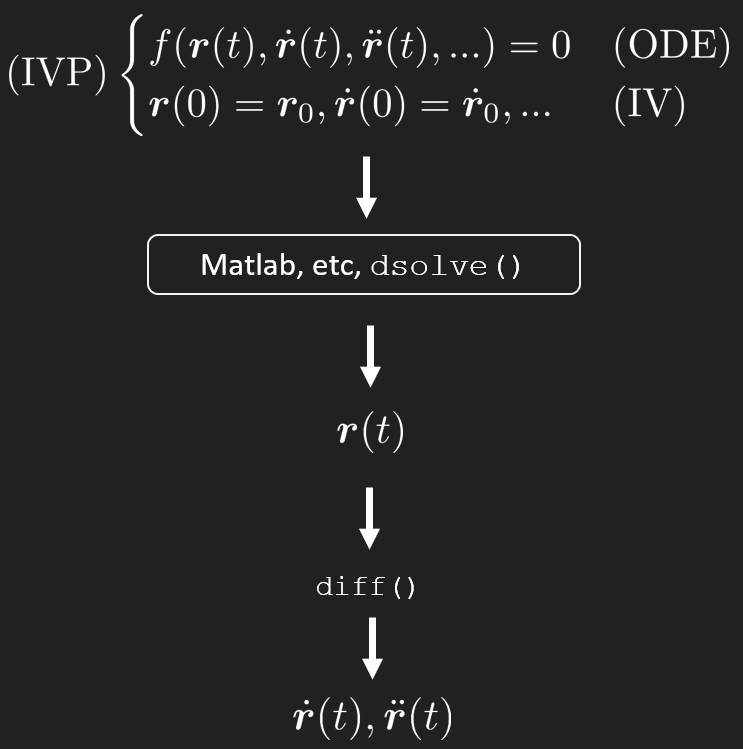
The modern workflow in computational dynamics can be summarized in the figure below
Workflow
To get between the different quantities position, \(\mathbb{r}(t)\), velocity \(\dot{\mathbb{r}}(t)\) and acceleration \(\ddot{\mathbb{r}}(t)\) we take the derivative in one direction and integrate in the other. In practice one does not typically manually integrate expressions, one typically solves an ordinary differential equation (ODE) instead, which takes us all the way down to \(\mathbb{r}(t)\) which is the solution to an ODE. Then we can take the derivative to determine the needed quantities. This is typical for a symbolic solution. Non-linear ODEs, on the other hand, are typically solved using various numerical algorithms which will first generate velocity, \(\dot{\mathbb{r}}\) on the way down to the final position \(\mathbb{r}\).
Newtonian physics is formulated as the kinetic equation
\[ \sum \mathbb{F} = m\ddot{\mathbb{r}} \]
which is a second order ODE, but in kinematics we se equally often differential equations of first order. Regardless, it is very convenient to solve any equation using a computational approach.
IVP
⚠ Note
The computational approach to dynamics is to formulate an initial value problem (IVP) and solve it using a differential equation solver.
We formulate an ODE which needs to be (at least piece-wise) valid for all \(t\) and apply initial conditions at the beginning of the analysis and/or at some other known state as boundary conditions (BC) to fix the unknown constants, where the number of constants depend on the order of the differential equation.
In this approach, the time \(t\) is the central parameter that ties the quantities (\(\mathbb{r}\), \(\dot{\mathbb{r}}\) and \(\ddot{\mathbb{r}}\)) together, which is why it often pops out in the solution without being maybe being explicitly asked for. This is the nature of Newtonian mechanics, it is inherently transient, meaning the state of the body is known for every time step. As we shall see in upcoming chapters, there are other methods which can greatly simplify calculations and modeling if the dependency of time is not important, e.g., 6.2.7. Note however that a complete dynamic analysis requires the solution of the ODE.
The inquiries to the model can be essentially divided into two categories:
Explicit time dependent, the equations are explicitly functions of a time variable, e.g., \(\dot{\mathbb{r}}(t)\), such that we can evaluate the quantities for a given time.
Implicit time dependent, where we want to know a quantity expressed as a function of another quantity and thus we need to solve an equation to get the time which is common for both quantities. E.g., find the velocity when the position is a given value, \(\dot{\mathbb{r}}(\mathbb{r})\).
Coordinate systems
Coordinate systems
There are several types of bases (or coordinate systems) on which we can formulate kinematic expressions and work with derivatives, traditionally this is done to simplify calculations, done by hand, and the resulting symbolic expressions.
⚠ Note
We can avoid this whole exercise of practicing to compute velocities and acceleration in various bases by just formulating relations in Cartesian coordinates and directly work with the position vector \(\mathbb{r}\) which can be easily projected onto any other bases if needed. Let the computer do the tedious mathematics!
We shall here derive the most common coordinate systems and their base vectors such that this projection can be done.
Cartesian, our typical xyz-system, here denoted, \(\mathbb{e}_x, \mathbb{e}_y, \mathbb{e}_z\), with \(\mathbb{e}_x = [1, 0, 0]^\mathsf{T}\), \(\mathbb{e}_y = [0, 1, 0]^\mathsf{T}\) and \(\mathbb{e}_z = [0, 0, 1]^\mathsf{T}\).
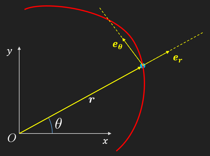
Polar or circular (2D) or cylindrical (3D), \(\mathbb{e}_r, \mathbb{e}_\theta, \mathbb{e}_z\).
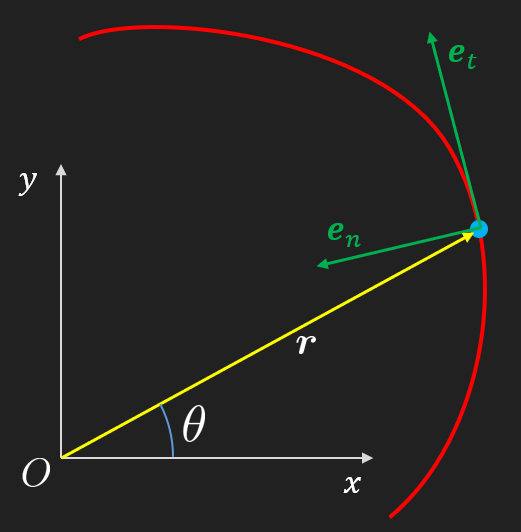
Natural (tangent, normal and bi-normal), \(\mathbb{e}_t, \mathbb{e}_n, \mathbb{e}_b\).
Sometimes the bases can be denoted simply \(\mathbb i, \mathbb j\) and \(\mathbb k\), but throughout this treatment we will try to be explicit and denote basis vectors and unit vectors with a specific sub-index for clarity.
Natural coordinates
The tangent vector \(\mathbb{e}_t\) is always pointing in the parameter direction, tangential to the path and is defined as the direction of the velocity
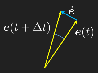
In order to ensure orthogonality of two vectors, we can take their dot product, if the resulting scalar is zero, they must be orthogonal. If two vectors are parallel then their dot product must be one, i.e., \(\mathbb{e} \cdot \mathbb{e} = 1\). Now we can take the time derivative of this expression \(\frac{d}{dt}(\mathbb{e} \cdot \mathbb{e} = 1) \stackrel{\text{product rule}}{=} \frac{d}{dt}\mathbb{e} \cdot \mathbb{e} + \mathbb{e} \cdot \frac{d}{dt}\mathbb{e} = 0 = \dot{\mathbb{e}} \cdot \mathbb{e} + \mathbb{e} \cdot \dot{\mathbb{e}} = 0 \Leftrightarrow \dot{\mathbb{e}} \cdot \mathbb{e} = 0 \Rightarrow \mathbb{e} \perp \dot{\mathbb{e}}\)
Also note that typically \(|\dot{\mathbb{e}}| \neq 1\).
Unit Vector Derivative
So at the limit \(\Delta t \to 0\) we clearly see that \(\mathbb{e} \perp \dot{\mathbb{e}}\).
Remark 1:
Let \(\mathbb{r}(t) = [\cos{\theta(t)}, \sin{\theta(t)}]\)
⚠ Note
Be careful when defining angles as degrees! Angles will be functions of time in what follow, meaning implicit derivation will yield expressions where angles are directly multiplied with distances or velocities, this only works if the angles are defined as radians!
We start by defining the angle as a function of time, \(\theta(t)\) and the position vector as a function of this angle.
What we computed above is the a scaled direction vector which is orthogonal to the direction vector \(\mathbb{e}_r\). Note that the time derivate of \(\theta\) appears from the implicit differentiation, which is why \(|\dot{\mathbb{e}}|\neq 1\) necessarily. In fact this is the angular velocity, \(\omega = \dot{\theta}\). The direction of rotation is the sign of \(\dot{\theta}\) i.e., {-1,1}.
The above we re-write in Newton notation and define the basis vector as \(\mathbb e_\theta\)
Here we can see that \(\frac{\dot{\theta}}{|\dot{\theta}|}\) only returns the sign of \(\dot{\theta}\). Thus in this example \(\mathbb{e}_\theta = [-\sin\theta, \cos\theta]^\mathsf T\) and we get
We shall here derive the kinematic equations explicitly in polar coordinates. Note again that in practice, working with a symbolic math manipulator like sympy, we can just formulate $ $ and \(\ddot{\mathbb r}\) in Cartesian coordinates and project onto the base. There is no need to learn the derived expressions below by heart in a modern workflow, instead we explore the connections between these entities and their physical meaning.
Polar coordinates
We begin by stating the earlier established bases.
and with \(\dot{\mathbb{e}}_r = \dot{\theta}\mathbb{e}_\theta\) and \(\dot{\mathbb{e}}_\theta = -\dot{\theta}\mathbb{e}_r\) we have the expression of the acceleration vector expressed in polar coordinates
Arguably more important are the kinematic relation expressed in Natural coordinates and even more useful are the acceleration terms which are split into normal and tangential directions. Here we shall derive these expressions explicitly, but note that we can always get these by just projecting the total velocity or acceleration vector onto any bases. Thus, there is no need to know these formulas or use them only for the sake of computing the quantities in one of these special bases.
Natural coordinates
We begin by stating the earlier established bases:
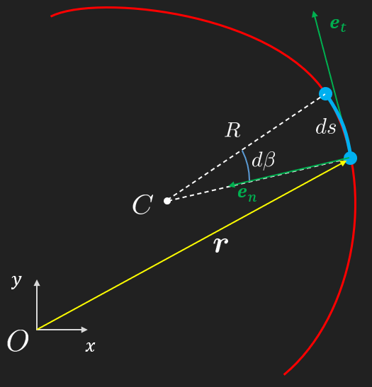
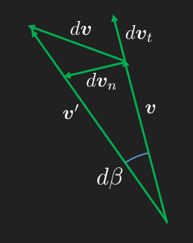
Next, we introduce the center of curvature, \(C\), at some point \(\mathbb{r}(t)\) and the corresponding curvature radius \(R\). We then can fit a circle arc length in the neighborhood of \(\mathbb{r}(t)\) such that we get a constant radius \(R\) for an infinitesimal circle arc angle \(d\beta\). This way we can get a relation between the section distance \(ds\) and the angle
Radius of curvature
This circle arc length relation, along with the Pythagorean theorem and trigonometry is a corner stone in dynamics and the main building blocks in our modelling toolbox.
Velocity in natural coordinates
We remember the definition of velocity as \(v = \frac{ds}{dt}\) and using the arc length relation we get
This relation is useful for when the angular rate \(\dot{\beta}\) is sought.
Angular rate
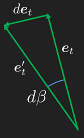
As seen in the figure above, a small change in the angle \(d\beta\) causes a corresponding change \(d\mathbb{e}_t\) in the unit tangent vector. The direction of \(d\mathbb{e}_t\) is perpendicular to \(\mathbb{e}_t\) and is defined as the normal direction \(\mathbb{e}_n\). We can thus formulate the relation:
We see from the figure above that the acceleration vector can be split into a tangential and a normal component, \(\ddot{\mathbb{r}} = a_t\mathbb{e}_t + a_n\mathbb{e}_n\). We can find these components by taking the time derivative of the velocity vector and using the product rule
From this expression we note that we always have an acceleration as long as there is non-zero velocity and a curved path.
This split into the normal and tangential directions will be revisited and used once we get to the kinetics chapter.
A tiny view on differential geometry
The theory of curves is an extensive topic within the field of differential geometry. Here, we will only introduce some basic concepts, such as the arc length. For a general curve, the arc length may not have a closed-form solution and is found by integrating the speed \(|\dot{\mathbb{r}}(t)|\):
\[
s(t) = \int_0^t |\dot{\mathbb{r}}(t)| dt
\]
Using the arc length \(s\) as the parameter instead of time \(t\) can sometimes lead to simpler expressions for derivatives. However, since \(s\) is itself a function of \(t\), this change of variable does not necessarily simplify computer-based calculations.
Another important concept is curvature, \(\kappa(t) = \frac{1}{R(t)}\). As expected, the curvature approaches zero as the radius of curvature \(R(t)\) tends to infinity, which corresponds to a straight path. The center of curvature, \(\mathbb{r}_C(t)\), is given by:
This point is the center of the osculating circle (a term coined by Leibniz as Circulus Osculans), which is the circle that best approximates the curve at a given point. Natural coordinates are particularly useful for this type of analysis.
⚠ Note
In the special case when \(R(t)\) is constant the bases of polar coordinates coincide with the bases of the natural coordinates.
The torsion of a curve, \(\tau(t)\), measures how sharply it twists out of its plane of curvature. A simple analogy is the pitch of a screw. The derivations for both curvature and torsion can be complex, see e.g., the Frenet-Serret formulas, so the formulas are stated here without proof:
where \(\dot{\ddot{\mathbb{r}}}\) denotes the third-order time derivative of the position vector, also known as jerk or jolt. For the names of higher-order derivatives, see this list.
Remark 2:
Let us work out the curvature and torsion on a simple example, let
\[
\mathbb{r}(t) = R [\cos(t), \sin(t), 0]^\mathsf{T}
\]
import sympy as spt = sp.symbols('t', real=True, positive=True)R = sp.symbols('R', real=True, positive=True)r = R * sp.Matrix([sp.cos(t), sp.sin(t), 0])r
# tau = - (r_dot x r_ddot) . r_dddot / |r_dot x r_ddot|^2# The cross product r_dot.cross(r_ddot) is not zero, so we can proceed.tau = sp.simplify(- (r_dot.cross(r_ddot)).dot(r_dddot) / (r_dot.cross(r_ddot)).norm()**2)tau
\(\displaystyle 0\)
The results seem reasonable, torsion is zero since the path is zero in the \(z\)-direction.
□
Osculating circle
Let’s define a path and find the necessary components for the osculating circle.
The path is given by: \[
\mathbb{r}(t) = [t, \sqrt{t}\sin(2t)]^\mathsf{T}
\]
Osculating Circle Animation
Code
import sympy as spimport numpy as npimport matplotlib.pyplot as pltfrom matplotlib.animation import FuncAnimation, PillowWriterfrom IPython.display import Image, display# Define the symbolic variablest = sp.Symbol('t')# Define the pathr = sp.Matrix([t, sp.sqrt(t)*sp.sin(2*t)])# Calculate derivativesr_dot = r.diff(t)r_ddot = r.diff(t, 2)# Calculate curvaturekappa = (r_dot[0]*r_ddot[1] - r_dot[1]*r_ddot[0]) / (r_dot[0]**2+ r_dot[1]**2)**(3/2)R =1/kappa# Calculate the normal vectore_t = r_dot / r_dot.norm()e_n = sp.Matrix([-e_t[1], e_t[0]])# Calculate the center of curvaturer_C = r + R*e_n# Lambdify the symbolic expressions for numerical evaluationr_func = sp.lambdify(t, r, 'numpy')r_C_func = sp.lambdify(t, r_C, 'numpy')R_func = sp.lambdify(t, R, 'numpy')e_t_func = sp.lambdify(t, e_t, 'numpy')# Set up the figure and axes for the animationfig, ax = plt.subplots(figsize=(8, 6))fig.patch.set_facecolor('#212121')ax.set_facecolor('#212121')ax.set_aspect('equal')ax.set_xlabel('x', color='white')ax.set_ylabel('y', color='white')ax.set_title('Osculating Circle Animation', color='white')ax.tick_params(axis='x', colors='white')ax.tick_params(axis='y', colors='white')for spine in ax.spines.values(): spine.set_edgecolor('white')# Define the time range for the animationt_vals = np.linspace(0.01, 10, 400)path = r_func(t_vals)# Plot the pathax.plot(path[0].flatten(), path[1].flatten(), 'c-', label='Path')# Initialize the plot elements to be animatedparticle, = ax.plot([], [], 'ro', label='Particle')circle_line, = ax.plot([], [], 'g-', label='Osculating Circle')tangent_arrow = ax.quiver(0, 0, 0, 0, color='b', scale=1, angles='xy', scale_units='xy', label='Tangent')radius_arrow = ax.quiver(0, 0, 0, 0, color='r', scale=1, angles='xy', scale_units='xy', label='Radius of Curvature')# Set the axis limitsax.set_xlim(0,10)ax.set_ylim(-3,3)#legend = ax.legend(loc='upper right')#legend.get_frame().set_facecolor('#424242')#for text in legend.get_texts():# text.set_color('white')ax.grid(False)# Animation update functiondef update(frame):# Get the current position, center of curvature, and radius pos = r_func(frame) center = r_C_func(frame) radius = R_func(frame) et = e_t_func(frame)# Update the particle's position particle.set_data(pos[0], pos[1])# Update the tangent arrow tangent_arrow.set_offsets(pos.flatten()) tangent_arrow.set_UVC(et[0], et[1])# Update the radius arrow radius_vector = center - pos norm_radius_vector = radius_vector / np.linalg.norm(radius_vector) radius_arrow.set_offsets(pos.flatten()) radius_arrow.set_UVC(norm_radius_vector[0], norm_radius_vector[1])# Generate the points for the osculating circle theta = np.linspace(0, 2* np.pi, 100) circle_x = center[0] + radius * np.cos(theta) circle_y = center[1] + radius * np.sin(theta) circle_line.set_data(circle_x, circle_y)return particle, circle_line, tangent_arrow, radius_arrow# Create the animationani = FuncAnimation(fig, update, frames=t_vals, blit=False, interval=50)# Save and display the animation as a GIFwriter = PillowWriter(fps=20)gif_path ="graphics/kinematics_osculating_circle.gif"ani.save(gif_path, writer=writer)plt.close(fig)
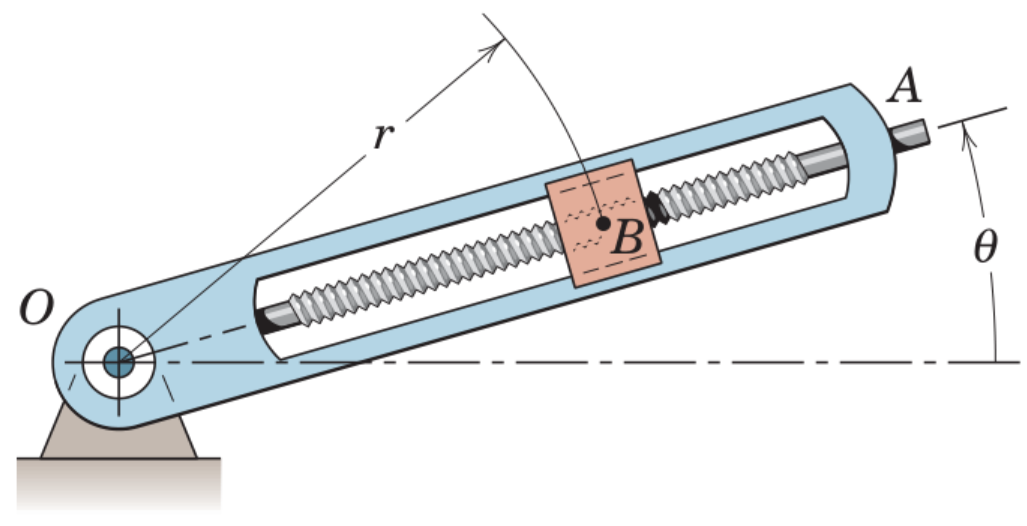
Circular motion
A special case of curvilinear motion is planar circular motion.
Let us study the case of a particle in polar coordinates using the arm below
We can clean up the expression by introducing the angular velocity in Newton notation, \(\dot{\theta} = \frac{d}{dt}\theta\) and the angular acceleration \(\ddot{\theta} = \frac{d^2}{dt^2}\theta\).
In the expression above, we made substitutions to make the expression more compact. Clearly we can handle tedious expressions like this using a computer algebra system.
where \(\mathbb{e}_\theta\) is perpendicular to \(\mathbb{e}_r\) and rotated 90 degrees counter-clockwise.
Now just project the Cartesian vectors onto the polar bases. We can just use the dot product to project onto the bases since the bases are orthonormal, i.e., \(|\mathbb e_r| = |\mathbb e_\theta| = 1\).
We get \(\mathbb{r}_{r\theta} = [\mathbb{e}_r \cdot \mathbb{r} , \mathbb{e}_\theta \cdot \mathbb{r} ]\).
The first term is the centripetal acceleration, always pointing towards the center of rotation, and the second term is the tangential acceleration, which is zero if the angular velocity is constant.
To summarize planar circular motion: with a constant \(r\), we have \(\dot{r} = \ddot{r} = 0\) and \(\mathbb{r} \perp \dot{\mathbb{r}}\) since \(\frac{d}{dt}(r^2) = 0 = \frac{d}{dt}(\mathbb{r} \cdot \mathbb{r}) = \dot{\mathbb{r}} \cdot \mathbb{r} + \mathbb{r} \cdot \dot{\mathbb{r}} \Leftrightarrow \mathbb{r} \cdot \dot{\mathbb{r}} = 0\). Note especially the centripetal acceleration\(-r\dot{\theta}^2\mathbb{e}_r\), it is directed in the negative direction of \(\mathbb{e}_r\), towards the center of the circle.
If the rotational velocity is constant, i.e., if \(\omega = \dot{\theta} = \text{constant}\) or \(\alpha = \ddot{\theta} = 0\) then we only have centripetal acceleration, caused by a curvilinear motion and perpendicular to the tangent direction, directed inwards, towards the center.
Another easy way is to explicitly rotate the base \(\mathbb{e}_r\) by 90 degrees into the direction of curvature, the drawback is we need to know which direction to rotate into, which is why the previous method is preferred, since the direction of rotation is determined by the sign of the angular velocity \(\omega\).
Relative motion
Relative motion
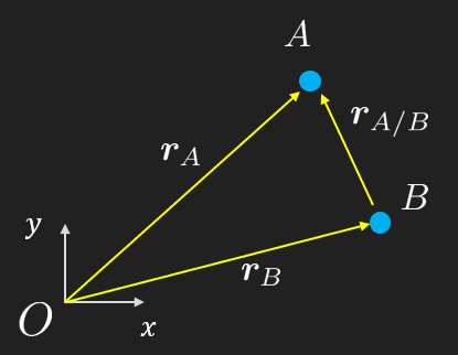
Many times we can express position and motion (velocities and acceleration) relative to some other point rather than the origin. This is done such that the modeling becomes significantly easier and less error prone. Besides, in real world applications, engineers need to make measurements and many times it is more accurate to make relative measurements rather than absolute. This approach is called relative motion analysis and will be used extensively in rigid body dynamics.
If we know the position of particle \(B\) as well as the relative position of particle \(A\) with respect to \(B\), that is \(\mathbb{r}_{A/B}\) (Can be read: A seen from B) we can express the absolute position of \(A\) as
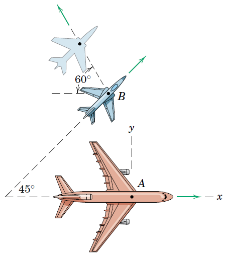
Passengers in the A380 flying east at a speed of 800 km/h observe a stunning JAS 39 Gripen passing underneath with a heading of 45\(^\circ\) in the north-east direction, although to the passengers it appears that the JAS is moving away at an angle of 60\(^\circ\) as shown in the figure. Determine the true velocity of the JAS 39 Gripen.
Solution
We have two unknows, the absolute speed of the JAS, \(v_B\) and the relative speed observed from the A380, \(v_{B/A}\).
We formulate the relative motion equation to suit our problem \[
\mathbb{v}_B = \mathbb{v}_A + \mathbb{v}_{B/A}
\]
Using the known directions we can express the matrix equation
To conclude, the JAS is moving away from the passengers at 586 km/h and its absolute speed is 717 km/h.
Example 2 - Data fitting
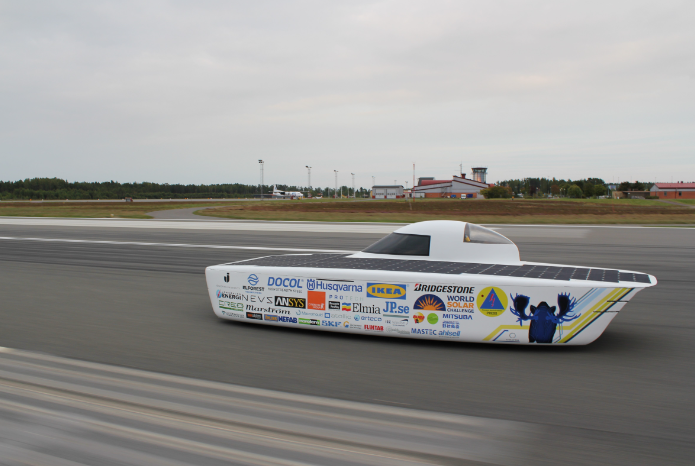
Solar Car
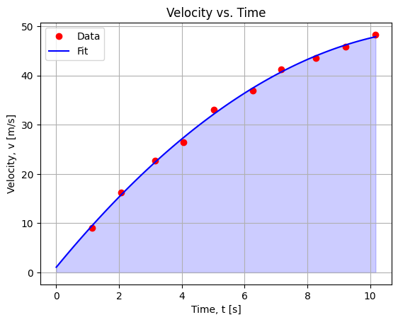
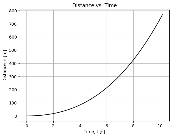
The acceleration performance of a new solar car is being tested at the Jönköping airfield. The JTH students are measuring time against velocity and the data is presented as two vectors. Create a suitable continuous function of the speed and determine how far the car has traveled at the last measurement point. Plot the distance - time curve as well as the acceleration curve.
\[v(t) = 1.05549793621106 t^{2} + 7.75454224391215 t - 0.309736757594531\]
We can also use the numpy.polyfit function which is a wrapper around numpy.linalg.lstsq and does the same thing, but is more convenient for polynomial fitting.
c = np.polyfit(T, V, 2)c
array([-0.30973676, 7.75454224, 1.05549794])
In the code below we can evaluate the fitted polynomial and its derivative using numpy.polyval.
Code
import matplotlib.pyplot as plt# Plot the data and the quadratic functionfig, ax = plt.subplots()ax.plot(T, V, 'ro', label='Data')tn = np.linspace(0, max(T), 100)vn = np.polyval(c, tn)ax.plot(tn, vn, 'b-', label='Fit')ax.set(xlabel='Time, t [s]', ylabel='Velocity, v [m/s]', title='Velocity vs. Time')ax.grid(True)ax.legend()ax.fill_between(tn, vn, color='b', alpha=0.2)plt.show()
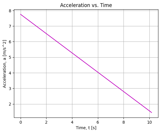
# Acceleration is the derivative of velocitya = sp.diff(v, t)
\[a(t) = 7.75454224391216 - 0.619473515189064 t\]
Code
# Plot accelerationan = sp.lambdify(t, a, 'numpy')(tn)fig, ax = plt.subplots()ax.plot(tn, an, 'm-')ax.set(xlabel='Time, t [s]', ylabel='Acceleration, a [m/s^2]', title='Acceleration vs. Time')ax.grid(True)plt.show()
# Total distance is the integral of velocitys_tot = sp.integrate(v, (t, 0, max(T)))
sn = sp.lambdify(t, s, 'numpy')(tn)fig, ax = plt.subplots()ax.plot(tn, sn, 'k-')ax.set(xlabel='Time, t [s]', ylabel='Distance, s [m]', title='Distance vs. Time')ax.grid(True)plt.show()
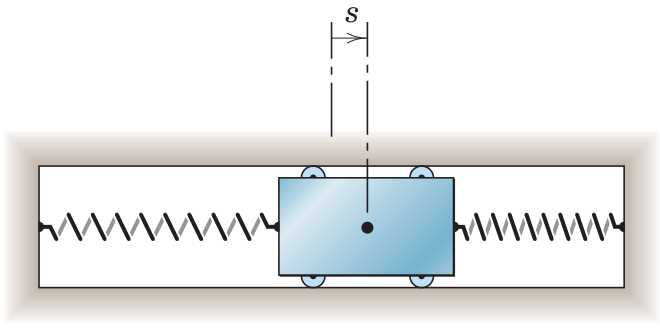
Example 3 - Oscillating slider
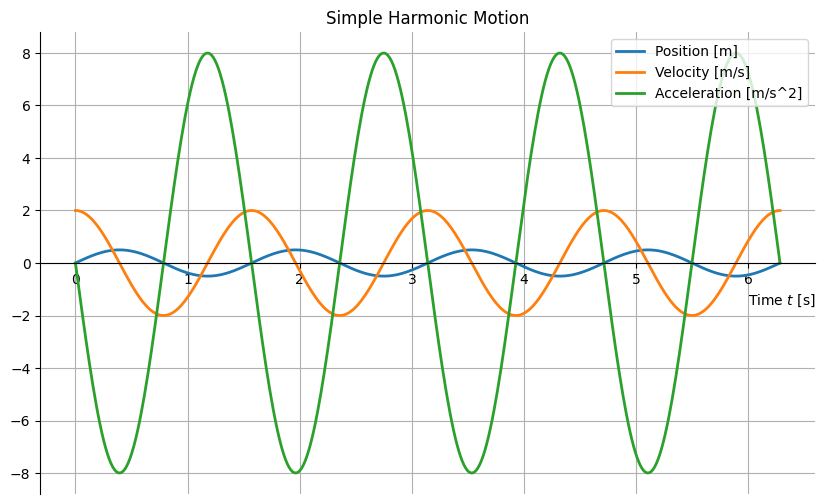
A spring mounted slider is being moved along the \(x\)-axis and has an initial velocity \(v_0=2 \mathrm{~m} / \mathrm{s}\) in the s-direction as it crosses the mid-position where \(s=0\) and \(t=0\). The two springs together exert a retarding force to the motion of the slider, which gives it an acceleration proportional to the displacement but oppositely directed and equal to \(a=-k^2 s\), where \(k=4\). Determine the displacement, velocity and acceleration of the slider and plot.
\(\displaystyle \frac{\sin{\left(4 t \right)}}{2}\)
Code
v_n = v_sol.subs(subs_data)v_n
\(\displaystyle 2 \cos{\left(4 t \right)}\)
Code
a_n = a_sol.subs(subs_data)a_n
\(\displaystyle - 8 \sin{\left(4 t \right)}\)
Code
t1 =2* np.pit_vals = np.linspace(0, t1, 400) # Create a range of time values for plotting# Lambdify converts a SymPy expression into a fast, callable numpy functionx_func = sp.lambdify(t, x_n, 'numpy')v_func = sp.lambdify(t, v_n, 'numpy')a_func = sp.lambdify(t, a_n, 'numpy')# Create the plotfig1, ax1 = plt.subplots(figsize=(10, 6))ax1.plot(t_vals, x_func(t_vals), linewidth=2, label='Position [m]')ax1.plot(t_vals, v_func(t_vals), linewidth=2, label='Velocity [m/s]')ax1.plot(t_vals, a_func(t_vals), linewidth=2, label='Acceleration [m/s^2]')# Set axis location to pass through the originax1.spines['bottom'].set_position('zero')ax1.spines['right'].set_color('none')ax1.spines['top'].set_color('none')ax1.set_xlabel('Time $t$ [s]', loc='right') # Using LaTeX for labelax1.legend()ax1.set_title('Simple Harmonic Motion')ax1.grid(True)
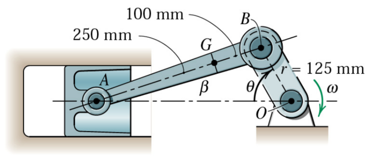
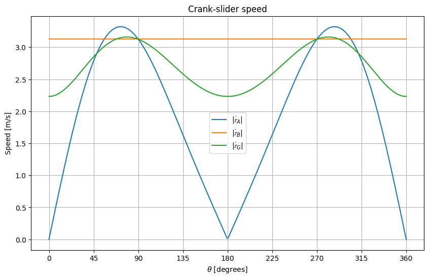
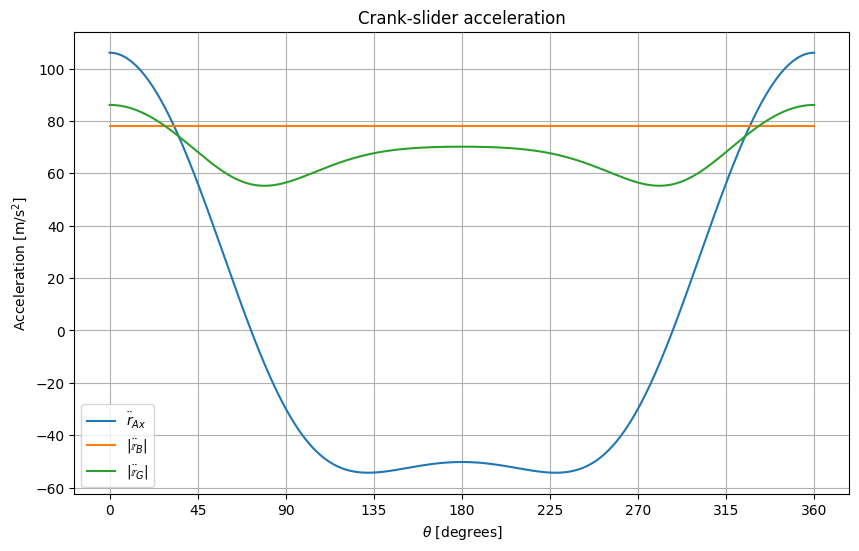
Example 3 - Crank slider mechanism
Crank Slider
Study the motion of the slider-crank mechanism. Plot the motion of A, G and B as well as their velocities and accelerations as a function of \(\theta\). Let the angular velocity \(\omega=25\) rad/s.