The method for solving problems in kinetics is an extension of statics and the methods used in the corresponding sections. Kinetics is the study of the relationship between forces and accelerations, and a starting point is Newton’s equation of motion
\[
\sum {\mathbb F}_i =m\;\mathbb a
\]
where \(\mathbb a\) is the center of mass (COM) of a body (or particle). For completeness, we shall here state the complete generalized equations of motion extended by Euler.
where \(\bar{I}\) is the moment of inertia for the body at the center of mass, otherwise known as the rotational inertia of a rigid body. We will give a proper introduction to this quantity in the section on rigid body kinetics. Note that the moment of inertia is given by the geometric relation
where \(\bar{\mathbb R}\) is the vector from the center of rotation (which in this case is the COM) to each point in the body.
Notice that in this general formulation we have \({\left\lbrack F_x ,F_y ,F_z \right\rbrack }^T =m\ddot{\mathbb r}\) and \({\left\lbrack M_x ,M_y ,M_z \right\rbrack }^T =\bar{I} \ddot{\theta}\), thus six equations (ODEs), where for each component we derive these equations by using a free body diagram, exactly as in statics. In order to get a specific solution to the system of equations, we need corresponding initial conditions and/or boundary conditions.
Suffice to say for now, if the body has a near-zero size, then \(\bar{\mathbb R}\to 0\) and we can assume particle dynamics and disregard the rotational part of the equation of motion, resulting in only three degrees of freedom instead of six. Similarly, if the rotational acceleration \(\ddot{\theta}\) is sufficiently low, we can assume particle dynamics. We will revisit the generalized equations of motion in rigid body kinetics.
Note that Newton’s second law of motion does not explicitly relate force to acceleration, but rather to momentum, paraphrased: “The time rate of change of a body’s momentum equals the force acting upon it,” i.e.,
Thus, we can create models where the body has a change of mass, e.g., rockets. When a body has constant mass, the expression reduces to what we are familiar with.
The solution of the equations of motion is typically done by solving a differential equation using either a symbolic or numerical solver. In traditional courses on classical mechanics, countless chapters are spent on deriving various analytical methods and formulas for simplifying problems or solving problems specifically designed to be solved using simple hand calculations. We shall here instead focus on solving problems completely and explicitly visualizing the whole motion.
Transient and state based solutions
We can apply two main methods for solving and analyzing dynamics problems. Transient, meaning we formulate an ODE and solve it either analytically of numerically. This gives us the position, velocity and acceleration vectors as a function of time over the complete time frame of interest. For situations where we are interested in solutions only at a perticular time (or state) we can formulate the problem as an energy equation instead using Langrangian or Hamiltonian formulation of mechanics. This can simplify the calculations drastically, since we do not need to iterate to the state from the inital state (using a numerical method) nor determine the accelerations or include forces that do no work.
A general workflow for a transient analysis can be summarized in the following steps:
Define a coordinate system:: Choose a suitable coordinate system (e.g., Cartesian, polar) that simplifies the problem.
Draw a Free-Body Diagram (FBD): Isolate the body or particle of interest and draw all the external forces acting on it, such as gravity, friction, normal forces, and applied loads.
Apply Equations of Motion: Use Newton’s second law (\(\sum \mathbb{F} = m\mathbb{a}\)) to write the equations of motion for each coordinate direction. This will result in a system of second-order ordinary differential equations (ODEs).
State Initial Conditions: To find a unique solution for the ODEs, you must specify the initial state of the system, which typically includes the initial position and initial velocity of the particle.
Solve the ODEs:
Analytically: For simpler problems, use symbolic mathematics tools (like SymPy’s dsolve) to find an exact mathematical expression for the position and velocity as a function of time.
Numerically: For more complex, non-linear problems where an analytical solution is not feasible, use numerical methods (like the Euler method or more advanced solvers) to approximate the solution at discrete time steps.
Analyze and Visualize: Use the solution to determine quantities of interest (e.g., maximum height, time of flight, final velocity). Plotting the position, velocity, and acceleration against time is often useful for visualizing the particle’s motion.
Example 1 - Linear friction
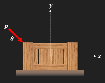
A box is being pushed from rest.
How much force \(P\) is required to accelerate the box to \(a_0 \;m/s^2\)?
What is the velocity of the box after \(t_1\) seconds?
How far does the box glide? At which time does it come to a stop?
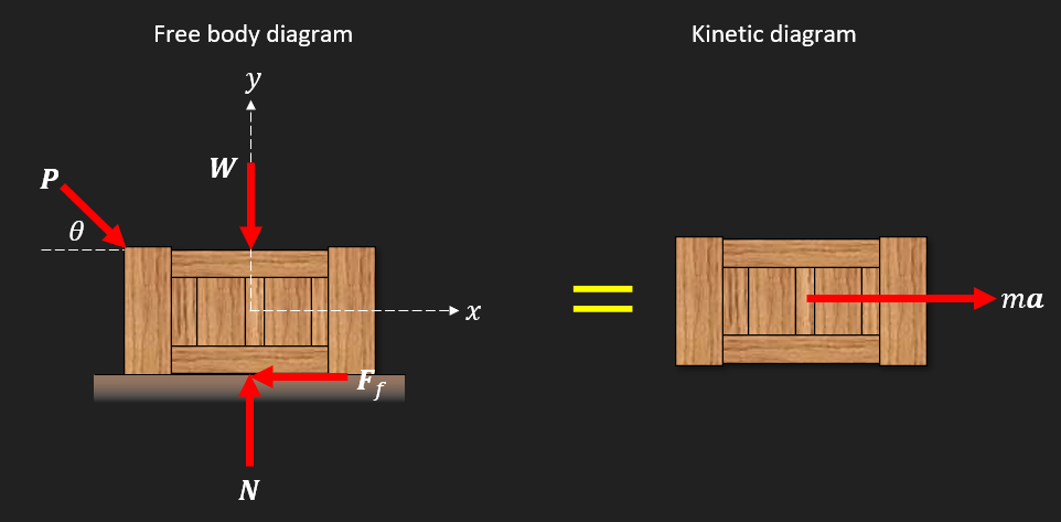
Step 1 - Free body diagram
# Define symbolic variablesmu_k, m, g, v_0, P, theta, N, a_x, t = sp.symbols('mu_k m g v_0 P theta N a_x t')x = sp.Function('x')(t)# Define vectors for the forces and accelerationF_ext = P * sp.Matrix([sp.cos(theta), -sp.sin(theta)])F_N = sp.Matrix([0, N])F_W = sp.Matrix([0, -m*g])F_f = sp.Matrix([-mu_k*N, 0])a = sp.Matrix([a_x, 0])# Newton's second law: sum of forces = m*aekv = sp.Eq(F_ext + F_N + F_W + F_f, m*a)ekv
\(\displaystyle \left[\begin{matrix}- N \mu_{k} + P \cos{\left(\theta \right)}\\N - P \sin{\left(\theta \right)} - g m\end{matrix}\right] = \left[\begin{matrix}a_{x} m\\0\end{matrix}\right]\)
Step 2 - Equations of motion
From the figure we get
\[
\begin{aligned}
& F_{\text {ext }}=P[\cos \theta,-\sin \theta]^\mathsf T \\
& F_N=[0, N]^\mathsf T \\
& F_W=[0,-m g]^\mathsf T \\
& F_f=\left[-\mu_k N, 0\right]^\mathsf T
\end{aligned}
\]
and the the acceleration vector is
\[
\boldsymbol{a}=\left[a_x, 0\right]^\mathsf T
\]
Using Newtons second law of motion we can formulate
\[\begin{gathered}
\sum F=m a \Rightarrow \\
P\left[\begin{array}{c}
\cos \theta \\
-\sin \theta
\end{array}\right]+\left[\begin{array}{c}
0 \\
N
\end{array}\right]+\left[\begin{array}{c}
0 \\
-m g
\end{array}\right]+\left[\begin{array}{c}
-\mu_k N \\
0
\end{array}\right]=\left[\begin{array}{c}
m a_x \\
0
\end{array}\right]
\end{gathered}\]
Step 3 - Solve for acceleration
From this equation system we need to solve for the same amount of unknowns as we have number of equations, we choose \(a_x\), of course, and \(N\) for the additional unknown. This is typical in mechanics to get additional unknowns, usually contact forces, or reaction forces. The choice is based on careful analysis of what is considered input parameter and what is an unknown quantity.
sol = sp.solve(ekv, (a_x, N), dict=True)[0]a_x_expr = sol[a_x]N_expr = sol[N]
\[\begin{align*}N &= P \sin{\left(\theta \right)} + g m \\[2.5ex]a_x &= - \frac{P \mu_{k} \sin{\left(\theta \right)}}{m} + \frac{P \cos{\left(\theta \right)}}{m} - g \mu_{k}\end{align*}\]
From the expression we can see that the vertical component of \(P\) causes additional friction in the negative x-direction whereas the horizontal component gives rise to an acceleration in the positive x-direction. Analyzing symbolic expressions before substitution is a good idea in the modeling stage, since we can verify the model much easier.
Step 4 - Formulating a set of differential equations (Kinematics)
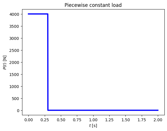
Let us assume that the box is given a push from \(P\) during a short time. Modeling a “push” can be interpretet in several way, we will start with the easy one first: The force is some constant value during a short period of time, i.e., let
In order to solve this problem we need to tackle this piecewise, we need to set up a differential equation with initial values for the range \(t \in[0,0.3] \mathrm{s}\) and another differential equation with initial values for the range \(t \in\left[0.3, t_{\text {end }}\right]\).
The strategy:
We can then formulate the differential equation and solve it to get the position \(x(t)\) which we can differentiate to get \(v(t)\). Then we can find out at what time the velocity is zero, \(t_{\text {end }}\), it is at this time that the box has come to stop.
⚠ Note
After \(t_{\text {end }}\) our friction model is no longer physical! That would mean that the box starts sliding backwards, which is absurd.