Parametric Involute Spur Gear in SolidWorks

Visualizing the involute

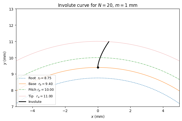
We plot the involute for a gear with \(N = 20\) and \(m = 1\,\text{mm}\), together with the four reference circles. The involute starts at the base circle and spirals outward; we draw it from \(\alpha = 0\) to the value of \(\alpha\) where it crosses the tip circle.

import numpy as np
import matplotlib.pyplot as plt

# Gear parameters
N = 20                          # Number of teeth
m = 1                           # Module (mm)
pressure_angle = np.radians(20) # Pressure angle

pitch_radius = m * N / 2
base_radius  = pitch_radius * np.cos(pressure_angle)
tip_radius   = m * (N + 2) / 2
root_radius  = pitch_radius - 1.25 * m

# Involute parameter at tip circle: solve |involute(alpha)| = tip_radius
# From the involute, the radial distance is r*sqrt(1 + alpha^2),
# so alpha_tip = sqrt((tip_radius/base_radius)^2 - 1)
alpha_tip = np.sqrt((tip_radius / base_radius)**2 - 1)

# Involute curve
alpha = np.linspace(0, alpha_tip, 300)
x_inv = base_radius * (np.sin(alpha) - alpha * np.cos(alpha))
y_inv = base_radius * (np.cos(alpha) + alpha * np.sin(alpha))

# Reference circles
theta = np.linspace(0, 2 * np.pi, 500)

fig, ax = plt.subplots(1, 1, figsize=(7, 7))
ax.set_aspect('equal')

for radius, label, ls in [
    (root_radius,  f'Root  $r_f = {root_radius:.2f}$',  '--'),
    (base_radius,  f'Base  $r_b = {base_radius:.2f}$',  '-'),
    (pitch_radius, f'Pitch $r_p = {pitch_radius:.2f}$', '-.'),
    (tip_radius,   f'Tip   $r_a = {tip_radius:.2f}$',   ':'),
]:
    ax.plot(radius * np.cos(theta), radius * np.sin(theta),
            ls=ls, lw=0.8, label=label)

ax.plot(x_inv, y_inv, 'k-', lw=2, label='Involute')
ax.plot(x_inv[0], y_inv[0], 'ko', ms=5)  # cusp at base circle

ax.set_title(f'Involute curve for $N={N}$, $m={m}$ mm')
ax.legend(loc='lower left', fontsize=9)
ax.set_xlabel('$x$ (mm)')
ax.set_ylabel('$y$ (mm)')
ax.set_xlim( -5*m, 5*m)
ax.set_ylim( pitch_radius - 3*m, pitch_radius + 3*m)
plt.tight_layout()
plt.show()

Derivation

At the base circle, the space between two adjacent tooth flanks has a half-width given by

\[ \frac{e_b}{2} = r_b \left( \frac{\pi}{2N} - \operatorname{inv}(\varphi) \right) \]

where \(\operatorname{inv}(\varphi) = \tan\varphi - \varphi\) is the involute function evaluated at the pressure angle (in radians). A fillet arc that fills a fraction \(k\) of this half-space (with \(k < 1\), e.g. \(k = 0.9\)) has radius

\[ R_f = k \, r_b \left( \frac{\pi}{2N} - \operatorname{inv}(\varphi) \right) \]

SolidWorks equation

"R_fillet" = 0.9 * "BR" * (pi / (2 * "N") - (tan("PressureAngle") - "PressureAngle" * pi / 180))

Important: Do not store \(\operatorname{inv}(\varphi)\) as a separate global variable. SolidWorks may assign it angular units (degrees), making it unusable in length expressions. By embedding the involute function directly in the fillet equation, the multiplication with BR (mm) forces the result into millimetres.

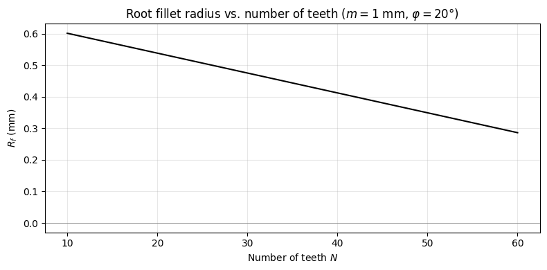
# Fillet radius as a function of N
N_range = np.arange(10, 61)
pitch_radii = m * N_range / 2
base_radii  = pitch_radii * np.cos(pressure_angle)
inv_phi     = np.tan(pressure_angle) - pressure_angle  # involute function
R_fillet    = 0.9 * base_radii * (np.pi / (2 * N_range) - inv_phi)

fig, ax = plt.subplots(figsize=(8, 4))
ax.plot(N_range, R_fillet, 'k-', lw=1.5)
ax.axhline(0, color='gray', lw=0.5)
ax.set_xlabel('Number of teeth $N$')
ax.set_ylabel('$R_f$ (mm)')
ax.set_title('Root fillet radius vs. number of teeth ($m = 1$ mm, $\\varphi = 20°$)')
ax.grid(True, alpha=0.3)
plt.tight_layout()
plt.show()

The problem

For a standard 20° pressure angle gear, the root circle falls below the base circle when \(N\) is small (roughly \(N < 34\)). In that case, the involute does not reach down to the root, and a straight radial line must bridge the gap between the root and base circles. For larger \(N\), the root circle lies above the base circle, the involute extends past the root, and this radial segment vanishes. If we draw the radial line and involute as separate sketch entities, the sketch topology changes when \(N\) crosses this threshold: the radial line disappears, any fillet referencing it breaks, and the model fails to rebuild.

The solution

We define one equation-driven curve that smoothly combines the radial line and the involute into a single entity. The parameter \(t\) runs from \(-1\) to \(1\). Internally, we define \(v = t \cdot t_{\text{tip}}\) (where \(t_{\text{tip}}\) is the involute parameter at the tip circle). When \(v \geq 0\) the involute trigonometric functions are active; when \(v < 0\) a straight radial line extends below the base circle. The curve always starts well below any possible root circle and always ends at the tip, regardless of \(N\).

Algebraic max and min without IF statements

SolidWorks equation-driven curves do not support IF, IIF, or max. We use the identity

\[ \max(v, 0) = \frac{v + \sqrt{v^2}}{2}, \qquad \min(v, 0) = \frac{v - \sqrt{v^2}}{2} \]

which evaluates to \(v\) or \(0\) depending on the sign of \(v\). In SolidWorks syntax: (v + sqr(v ^ 2)) / 2 and (v - sqr(v ^ 2)) / 2.

Curve equations

With the shorthand \(v = t \cdot t_{\text{tip}}\) and writing \(v^+ = \max(v, 0)\), \(v^- = \min(v, 0)\), the curve is

\[ x(t) = r_b \bigl[\sin(v^+) - v^+ \cos(v^+)\bigr] \]

\[ y(t) = r_b \bigl[\cos(v^+) + v^+ \sin(v^+)\bigr] + v^- \cdot r_b \]

The first terms are the standard involute evaluated at \(v^+\). When \(v < 0\), we have \(v^+ = 0\) and the involute terms reduce to \((0, r_b)\), i.e. the cusp point on the base circle. The \(v^- \cdot r_b\) term then adds a downward radial offset from the cusp, producing a straight line along the \(y\)-axis below the base circle. When \(v \geq 0\), we have \(v^- = 0\) and the curve is the involute.

SolidWorks equation-driven curve

Set the parameter range to \(t_1 = -1\), \(t_2 = 1\) and enter:

x(t):

"BR" * (sin(((t * "t_tip") + sqr((t * "t_tip") ^ 2)) / 2) - ((t * "t_tip") + sqr((t * "t_tip") ^ 2)) / 2 * cos(((t * "t_tip") + sqr((t * "t_tip") ^ 2)) / 2))

y(t):

"BR" * (cos(((t * "t_tip") + sqr((t * "t_tip") ^ 2)) / 2) + ((t * "t_tip") + sqr((t * "t_tip") ^ 2)) / 2 * sin(((t * "t_tip") + sqr((t * "t_tip") ^ 2)) / 2)) + ((t * "t_tip") - sqr((t * "t_tip") ^ 2)) / 2 * "BR"

The curve is one continuous entity from well below the root to the tip. The topology never changes.

Visualizing the unified curve

We plot the unified curve for several values of \(N\) to illustrate how it handles both small and large tooth counts. For each case, the root circle is shown as a dashed arc. When the root circle lies below the base circle, the straight-line portion of the curve is visible; when it lies above, the curve is purely involute down to the root.

from gear_geometry import unified_curve, gear_radii

fig, axes = plt.subplots(1, 4, figsize=(18, 5))

for ax, N_val in zip(axes, [12, 20, 40, 50]):
    pr, br, tr, rr = gear_radii(N_val, m)
    t_tip_val = np.sqrt((tr / br)**2 - 1)

    t_param = np.linspace(-1, 1, 1000)
    xc, yc = unified_curve(t_param, br, t_tip_val)

    ax.set_aspect('equal')
    ax.plot(xc, yc, 'k-', lw=1.5, label='Unified curve')

    # Reference circles (partial arcs near the tooth)
    arc = np.linspace(-0.15, 0.15, 200)
    for radius, lbl, ls in [(rr, 'Root', '--'), (br, 'Base', '-'),
                             (pr, 'Pitch', '-.'), (tr, 'Tip', ':')]:
        ax.plot(radius * np.sin(arc), radius * np.cos(arc), ls=ls, lw=0.7, label=lbl)

    status = "root < base" if rr < br else "root > base"
    ax.set_title(f'$N = {N_val}$ ({status})', fontsize=11)
    ax.legend(fontsize=7, loc='lower left')
    ax.set_xlabel('$x$ (mm)')
    ax.set_ylabel('$y$ (mm)')

plt.suptitle('Unified curve for different tooth counts ($m = 1$ mm)', fontsize=13)
plt.tight_layout()
plt.show()

Reference geometry

Before sketching the tooth profile, create four construction circles at RootRadius, BR, PitchRadius, and TipRadius. These serve as visual references and provide intersection points for trimming. Next, draw a reference line from the centre of the gear to the point where the involute crosses the pitch circle. Finally, define a midline reference: the variable MidAngle = 360 / (N * 4) gives the angular half-width of one tooth space at the pitch circle. Create a reference plane through the gear axis, rotated by MidAngle from the reference line. This plane will serve as the mirror plane when completing the full tooth space.

The three sketch entities

The half-tooth-space sketch always consists of exactly three entities:

1. The unified curve defined above, with parameter range \(t_1 = -1\), \(t_2 = 1\).
2. A root arc drawn as a centerpoint arc at radius RootRadius.
3. A midline closure along the tooth space midline, connecting the root arc to the tip circle (or back to the centre).

Trimming and filleting

Trim the unified curve below the root arc and trim the root arc beyond the midline. The result is a clean half-tooth-space profile forming a closed loop. At the corner where the trimmed curve meets the root arc, apply a sketch fillet with radius R_fillet. This corner always exists because the curve and root arc are always present as two distinct entities meeting at one point, regardless of the value of \(N\).