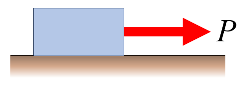
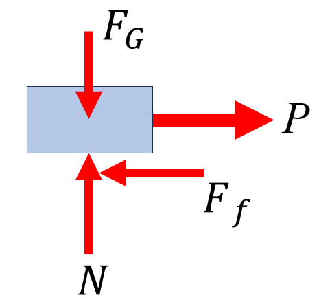
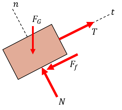
The box with the mass \(m\) kg is exposed to an external force \(P\) according to the left figure. Doing a free body diagram and applying Newton’s third law reveals a force \(F\) acting opposite to \(P\) along the contact surface. The magnitude of this friction force depends on the type of surface and the normal force \(N\). The relation between the normal force and friction force can be modelled using the Coulombs law:
\[
\boxed{ F \leq \mu_s N }
\]
where \(\mu_s\) is known as the static coefficient of friction. Coulomb developed a friction theory in the 1700 s for dry friction. This model assumes a linear relationship between \(F\) and \(N\) and even if we can empirically show that this does not generally hold for an arbitrarily large \(N\), Coulombs law is taken to be “good enough” for most situations, but should be used with care.
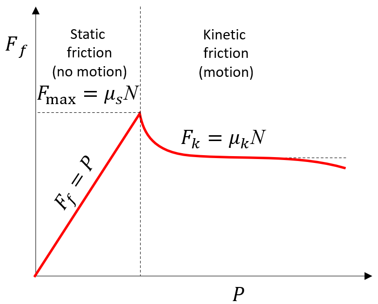
Figure 5.6.2: Relation between the external force \(P\) and friction force \(F_f\).
As the force \(P\) exceeds the largest possible frictional force \(F_{\max }\) the box will start to slide and get an acceleration, thus the model transitions to what is known as kinetic friction and the opposing force is given by \(F_k=\mu_k N\), where \(\mu_k\) is the kinetic coefficient of friction. This is where statics ends and dynamics continues.
The coefficients of friction can be calculated from empirical observations using measurements of forces, positions or angles.
⚠ Note
Any list containing the coefficient will be approximate, good accuracy is application dependent and must be measured.
Here is a list for (a rough) reference
Material
\(\mu_s\)
\(\mu_k\)
Steel on steel
\(0.1-0.3\)
\(0.03-0.3\)
Steel on wood
\(0.5-0.7\)
\(0.2-0.5\)
Leather on metal
\(0.3-0.6\)
\(0.2-0.3\)
Break pad on cast iron
0.4
0.3
Hemp rope on steel
0.3
0.2
Teflon on Teflon
0.05
0.05
Rubber on metal
\(0.4-0.5\)
\(0.3-0.4\)
Rubber on asphalt
\(0.7-1.0\)
\(0.5-0.8\)
Rubber on ice
0.1
0.05
⚠ Note
Note that Coulombs law is a very simple model in the world of tribology. Many applications need more sophisticated models of friction.
⚠ Note
For any problem involving rough surfaces where frictional forces need to be taken into account one needs to determine if the bodies are at rest or sliding. In general there are several types of states in contact points on a body. If we have a friction coefficient \(\mu_s\) and have the situation
\(F<\mu_s N\) then static equilibrium is possible since the surfaces can generate the needed friction force that is required for static friction.
\(F=\mu_s N\) then static equilibrium is still possible. This is a limit, often we write \(F_{\max }=\mu_s N\), to show that this is the maximum friction force, this limit is also known as fully established friction.
\(F>\mu_s N\) then static equilibrium is impossible. The surfaces cannot produce the frictional force that is required to keep static equilibrium. The body begins to slide, accelerates and we get dynamic equilibrium \(F=\mu_k N\), at this point the problem is transitioned into a dynamic problem and we have \(\Sigma F=m a\).
The basic rule for analysis with friction is that the frictional force-vector \(\bm F\) is set to be in the direction that opposes potential movement.
Essentially there two types of problem statements
All external forces except friction forces are known and we need to determine if the friction force can balance the external forces. This means that we need to check if \(F \leq \mu_s N\) in the contact surface, otherwise we have sliding and the problem is a dynamic problem with \(F=\mu_k N\).
Some external forces are unknown and we want to know how much more we can load the body until sliding occurs. This means that we add \(F_i=\mu_s N_i\) to all rough contact points and include these friction equations in the equilibrium equations. Solving for the unknown forces to answer the problem statement.
We show some typical examples involving friction.
Example 1: A box on a slope
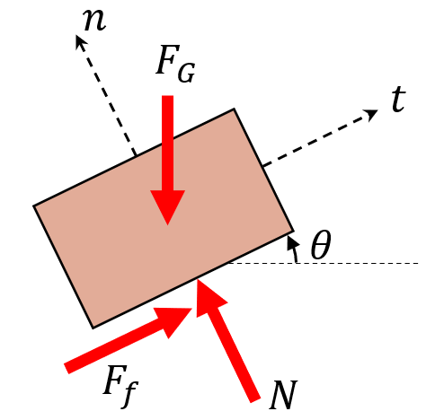
Determine the maximum angle \(\theta\) for which the box with mass \(m\) will not slide down the slope. The coefficient of static friction between the surfaces is \(\mu_s\).
Solution
FBD
Since we’re using a CAS, we can establish a normal coordinate system using the tangential direction \(t\) and the normal direction \(n\) to the slope. Once these directions are established we can easily express the force vectors in these directions and pose the equations of equilibrium.
We have equilibrium equations and an additional friction equation \(F_{\max }=\mu_s N\). Then we just solve for as many variables as we have equations.
The direction vector in the tangential direction is given by
\[ {\def\arraystretch{1.2}\left[\begin{matrix}F_{f} \cos{\left(\theta \right)} - N \sin{\left(\theta \right)}\\F_{f} \sin{\left(\theta \right)} + N \cos{\left(\theta \right)} - g m\\0\end{matrix}\right] = \left[\begin{matrix}0\\0\\0\end{matrix}\right]} \]
Additionally we have the friction equation
ekv2 = sp.Eq(F_f, mu*N)
\[ {\def\arraystretch{1.0}F_{f} = N \mu} \]
All together we have three equations and three unknowns. We can solve for the unknowns using SymPy.
sol = sp.solve([ekv1, ekv2], [F_f, N, mu], dict=True)[0]sol | la
\[ \begin{aligned}
F_{f} &= g m \sin{\left(\theta \right)} \\[9.0pt]
N &= g m \cos{\left(\theta \right)} \\[9.0pt]
\mu &= \tan{\left(\theta \right)}
\end{aligned} \]
Here we have that \(\theta = \tan^{-1}(\mu_s)\), also known as the angle of friction.
⚠ Note
A note for SymPy solve function. There are a number of ways solve returns solutions. For unique solutions we expect a list of one element containing a dict. Sometimes we just get the dict. One needs to check the output and use correct syntax to extract the solution.
In the above case we get a list with one element, which is a dict. First we need to index into the list and grab index 0 then we have the dict.
Note also that we explicitly use dict=True to get a dict as output. This should be the default behaviour of SymPy. But not always. In this case for unknown reasons, if omitted, we would get a list of solutions instead and not a dict.
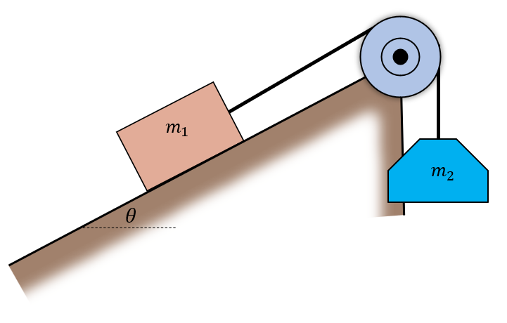
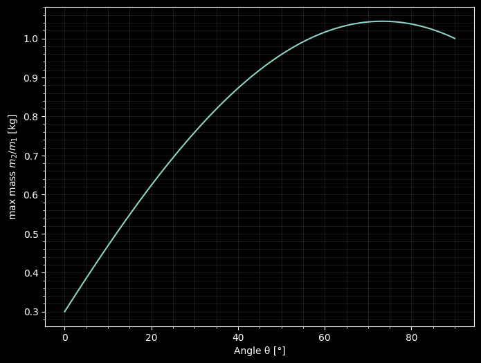
Two masses are rigged according to the figure. In what interval does \(m_2\) need to be in to prevent sliding of \(m_1\). Let \(\mu_s=0.3\) and \(\theta=20^{\circ}\).
Solution - Reformulation of the problem
We need to ensure that we understand the problem. This is imperitive to solve any engineering problem correctly. If in doubt, ask the problem owner for a clarification.
Let’s break down the above problem statement:
We \(m_2\) need to find the interval of \(m_2\) such that \(m_1\) does not slide. This means that we need to find the maximum and minimum values of \(m_2\) such that \(m_1\) is in static equilibrium. In other words:
Find
\[
m_{2, \min} < m_2 < m_{2, \max}
\]
such that \(m_1\) is in static equilibrium.
This gives rise to two cases: depending on if the box is just about to start gliding up or down. These cases result in two FBDs where the direction of the friction force is opposing the direction of movement.
Case 1: \(m_1\) is just about to start sliding down, i.e., finding \(m_{2\min}\)
An assumption we make is that the force \(T\) is transmitted through the pulley without any losses. This means that the tension in the rope is constant. We can also assume that the mass of the rope is negligible. This means that the tension in the rope is constant and equal to \(m_2 g\).
Kinematics
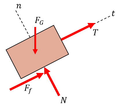
We need to establish the directions \(t\) and \(n\). Starting with the tangential direction \(t\) we have
\[
\bm e_t = [\cos \theta, \sin \theta, 0]^\mathsf T
\] The normal direction is given by \[
\bm e_n = [\cos \theta + 90^\circ, \sin \theta + 90^\circ, 0]^\mathsf T
\]
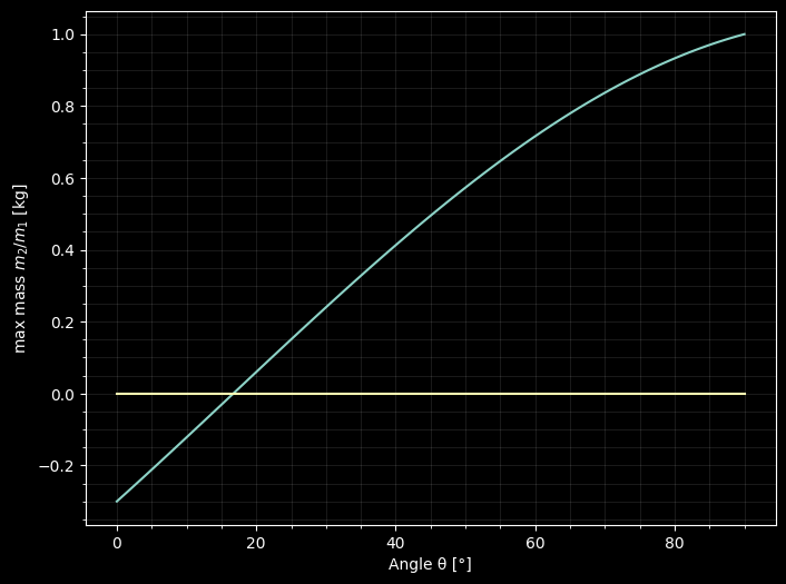
Feasibility analysis: At close to \(90^{\circ}\) the frictional force is so small that we get \(m_1=m_2\). At zero degrees the model does not work since we would get negative masses. Case 1 does not exists below slopes of ca \(17^{\circ}\), i.e., the box cannot slide downwards if the slope is less than \(17^{\circ}\).
Case 2: \(m_1\) is just about to start sliding up, i.e., finding \(m_{2\max}\)
In this case we have the following forces, with the friction force being reversed
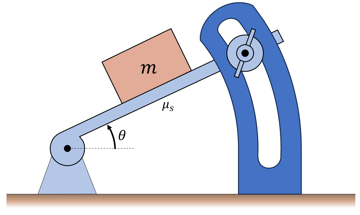
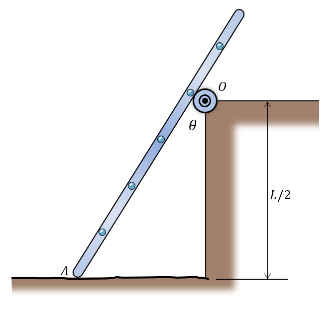
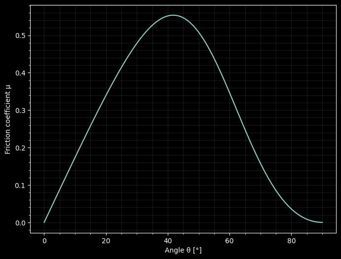
Determine the least possible \(\mu_s(\theta)\) at \(A\) such that the homogenous rod with a mass of \(m\) does not slide. There is no friction at \(O\). Disregard the radius of the roller at O. Draw a graph of \(\mu_s(\theta)\) for valid angles.
Solution
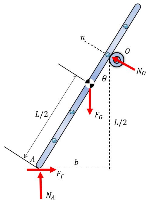
FBD
We start by defining the kinematics, the position of \(A\) needs to be defined as a function of that angle \(\theta\). Using trigonometry we recognize the triangle and have
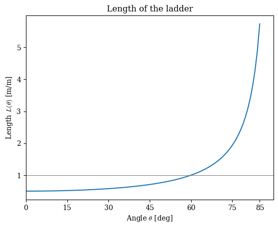
As seen from the ladder length graph, we cannot go beyond \(60^\circ\). This can also be verified using a sketch in CAD
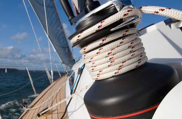
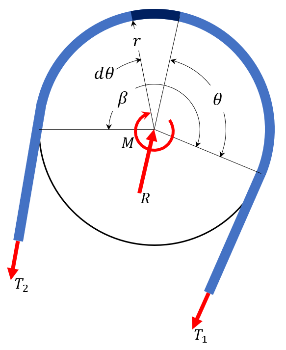
Example 4 - Flexible belts (Capstan equation)
Ropes and belts which are wrapped around cylinders are a very common application for static friction in mechanics. We shall look closer at the problem.
Free body diagram
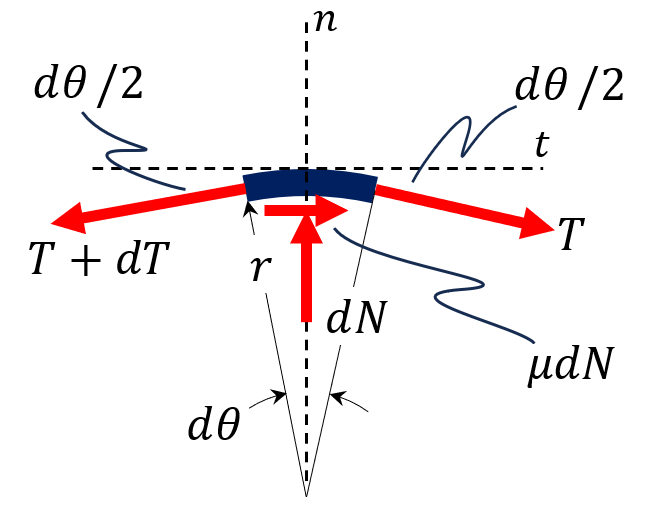
Infinitesimal belt element
Figure 5.6.6: Flexible belt free body diagram
A rope is wrapped some angle \(\beta \in[0, \infty]\) radians around a cylinder. We cut a small piece \(d \theta\) at an arbitrary angle \(\theta \in[0, \infty]\) and create a FBD according to the figure. We are interested in the maximum force and examine the limit just before sliding. The force equilibrium is divided into a tangential \((t)\) and radial \((n)\) direction
Since both dT and \(d \theta\) are very small, their product is even smaller and can be neglected, i.e., \(dTd \theta \ll dT, d \theta\)
Thus we end up with
\[
\left\{\begin{array}{l}
\mu dN=dT \\
dN=T d \theta
\end{array}\right.
\]
Eliminating \(dN\) and moving things around we can formulate a simple ordinary differential equation
\[
\frac{dT_2}{d \theta}=\mu T_2
\]
with the boundary condition \(T_2(0)=T_1\)
For which we can easily get the solution using SymPy symbolic differential equation solver dsolve:
import sympy as spfrom sympy import difftheta, mu, T1 = sp.symbols('theta, mu, T1', real=True)# Here we define the function T2T2 = sp.Function('T2')T2(theta)
\(\displaystyle T_{2}{\left(\theta \right)}\)
# Define the Differential EquationDE = sp.Eq(diff(T2(theta), theta), mu * T2(theta))DE
Ok, so with, e.g., \(\mu_s=0.25\) (hamp against steel according to some table) and wrapped five times we get
from sympy import exp, pimu =0.25T2 = T1 * exp(mu*5*2*pi)T2.evalf(6)
\(\displaystyle 2575.97 T_{1}\)
We see that the force \(T_2\) needs to be over 2500 times larger than \(T_1\) to be in balance. The Capstan equation (5.6.1) is extremely useful in many applications, e.g., belt breaking, winches, cranes, gearboxes, etc.
For a cool application see this video by Aaed Musa:
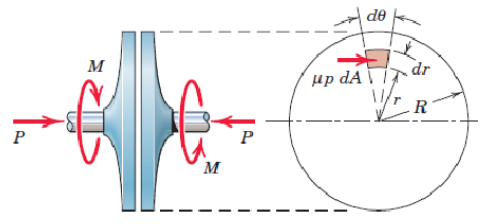
Example 5 – Clutch
A clutch transfers torque between two rotating shafts through friction. Two flat plates are pressed together by an axial force \(P\), and the friction between the contact surfaces transmits a moment \(M\). We want to relate the transmittable moment to the applied force, the friction coefficient, and the radius of the clutch face.
We integrate over the disk to get the total normal force and moment. A thin ring at radius \(r\) and width \(dr\) has area \(dA = 2\pi r\, dr\). If the contact pressure \(p\) is uniform across the disk, the normal force on the ring is \(dP = p\, dA\), the friction force is \(dF = \mu\, dP\), and the moment about the axis is \(dM = r\, dF\). Integrating from \(0\) to \(R\) gives the total \(P\) and \(M\), and from there we solve for the moment in terms of the applied force.
r, R_i, R_o, p, P, M = sp.symbols('r R_i R_o p P M', positive=True)mu = sp.Symbol('mu', positive=True)# Differential contributions over an annulus at radius rdA =2*sp.pi*rdP = p*dAdF = mu*dPdM = r*dF{'dA': dA, 'dP': dP, 'dF': dF, 'dM': dM} | la
\[ \begin{aligned}
dA &= 2 \pi r \\[9.0pt]
dP &= 2 \pi p r \\[9.0pt]
dF &= 2 \pi \mu p r \\[9.0pt]
dM &= 2 \pi \mu p r^{2}
\end{aligned} \]
Code
# Integrate from R_i to R_oP_total = sp.integrate(dP, (r, R_i, R_o))M_total = sp.integrate(dM, (r, R_i, R_o)){sp.Symbol('P'): P_total, sp.Symbol('M'): M_total} | la
\[ \begin{aligned}
P &= - \pi R_{i}^{2} p + \pi R_{o}^{2} p \\[9.0pt]
M &= - \dfrac{2 \pi R_{i}^{3} \mu p}{3} + \dfrac{2 \pi R_{o}^{3} \mu p}{3}
\end{aligned} \]
No we can solve for \(M\) and \(p\)
Code
sol = sp.solve([sp.Eq(P_total, P), sp.Eq(M_total, M)], [M, p])sol | la
\[ \begin{aligned}
M &= \dfrac{2 P R_{i}^{2} \mu + 2 P R_{i} R_{o} \mu + 2 P R_{o}^{2} \mu}{3 R_{i} + 3 R_{o}} \\[9.0pt]
p &= - \dfrac{P}{\pi R_{i}^{2} - \pi R_{o}^{2}}
\end{aligned} \]
The transmittable moment is \(M = \tfrac{2}{3}\mu P R\) and the contact pressure is \(p = P/(\pi R^2)\). The pressure relation is just the definition of pressure (force over area), and the moment scales linearly with \(\mu\), \(P\), and \(R\) as a quick dimension check confirms. Real clutches use multiple friction surfaces in series to multiply \(M\) without enlarging \(R\).
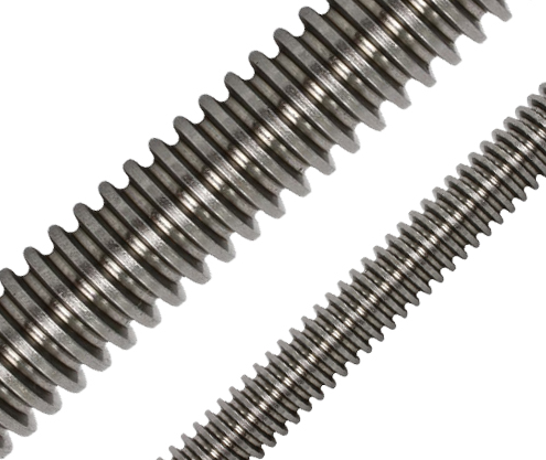
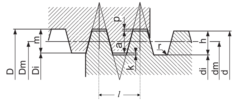
Example 6 – Screws
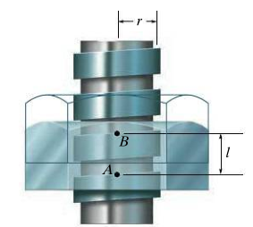
A screw converts rotation into linear motion (or, depending on use, transfers an axial load through a rotational input). A trapezoidal screw maximizes efficient transfer of torque to linear force, while a standard machine screw is shaped to maximize axial load capacity. Regardless of profile the analysis is the same: unwrap one revolution of the thread into a straight inclined plane, and the problem reduces to a block on a slope under friction.
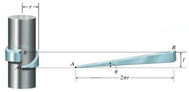
The pitch is the height the screw advances per revolution. Unwrapping one full thread along its mean radius gives a triangle whose hypotenuse is the thread, whose horizontal leg is \(2\pi r\) (the circumference at the mean radius), and whose vertical leg is the pitch. The thread angle \(\theta\) above the horizontal is \(\tan\theta = \text{pitch}/(2\pi r)\).
Trapezoidal screws have a larger pitch than standard machine screws, which makes them more efficient at converting rotation into linear motion at the cost of holding capacity. Ball screws reduce friction further with rolling contact at the cost of self-locking: an axial load can easily back-drive a ball screw, so a motor torque is required to hold position. Even trapezoidal screws can be back-driven given enough axial force. Machine screws on the other hand are self locking and cannot be back-driven. Pitch values for trapezoidal screws are tabulated by suppliers, e.g. mekanex.
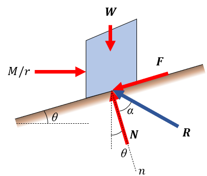
Mechanical analysis
We isolate a small segment of the thread and treat it as a block on the unwrapped incline. The thread angle \(\theta\) is the helix angle: \(\tan\theta = \text{pitch}/(2\pi r)\). The friction angle \(\alpha\) is defined by \(\tan\alpha = \mu\), so the contact reaction \(\bm R = \bm N + \bm F\) makes angle \(\alpha\) with the surface normal whenever the block is on the verge of sliding.
Three situations matter:
Raising a load: we apply torque to push the screw upward against the load.
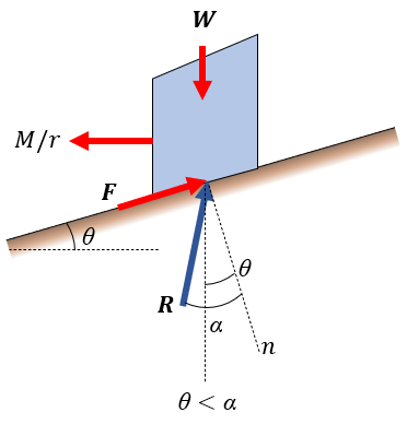
Lowering when \(\theta < \alpha\): the screw is self-locking, the load alone cannot drive it. To lower, we must apply torque in the opposite direction.
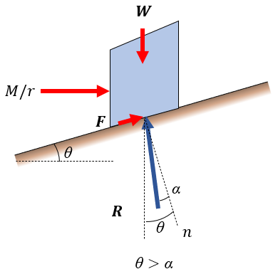
Self-unwinding when \(\theta > \alpha\): the thread is steep enough that the load alone overcomes friction. To hold the load we must apply torque in the lifting direction.
In all cases the analysis is the same FBD with three forces \(\bm W\), \(\bm F\), \(\bm N\) and an applied tangential force \(M/r\). Only the direction of friction (and of \(M/r\)) changes between cases.
Raising the load
Raising the load
The block slides up the incline, friction \(F = \mu N\) acts down the incline opposing the motion, and we push horizontally with \(M/r\) in the raising direction. Force balance gives three equations for the three unknowns \(M\), \(N\), \(F\).
M, N, F = sp.symbols('M N F', positive=True)W, r, theta, alpha = sp.symbols('W r theta alpha', positive=True)mu = sp.tan(alpha)eq1 = sp.Eq(M/r - F*sp.cos(theta) - N*sp.sin(theta), 0) # horizontaleq2 = sp.Eq(N*sp.cos(theta) - W - F*sp.sin(theta), 0) # verticaleq3 = sp.Eq(F, mu*N) # Coulomb
[eq1, eq2, eq3] | la.arraystretch(2.0)
\[ {\def\arraystretch{2.0}\begin{bmatrix}
- F \cos{\left(\theta \right)} + \dfrac{M}{r} - N \sin{\left(\theta \right)} = 0 \\
- F \sin{\left(\theta \right)} + N \cos{\left(\theta \right)} - W = 0 \\
F = N \tan{\left(\alpha \right)}
\end{bmatrix}} \]
sol_raise = sp.solve([eq1, eq2, eq3], [M, N, F])sol_raise | la
The torque needed to raise the load increases with both the thread angle (steeper thread, more axial advance per turn) and the friction angle (more friction, more loss). The denominator \(\cos(\theta+\alpha)\) vanishes when \(\theta + \alpha = \pi/2\), the geometric limit where any further increase in either angle would require infinite torque to lift.
Lowering the load when \(\theta < \alpha\)
Lowering when \(\theta < \alpha\)
When the thread angle is smaller than the friction angle, friction alone is enough to hold the load. The screw is self-locking: it will not unwind on its own. To make the load go down we must actively push the screw in the lowering direction. Friction now acts up the incline (opposing the lowering motion), and the applied tangential force \(M/r\) points the other way.
M_low = sp.symbols('M_low', positive=True)N_low, F_low = sp.symbols('N_low F_low', positive=True)# M/r now points in the lowering direction (negative x), friction reverses (now up the incline)eq1 = sp.Eq(-M_low/r + F_low*sp.cos(theta) - N_low*sp.sin(theta), 0)eq2 = sp.Eq(N_low*sp.cos(theta) - W + F_low*sp.sin(theta), 0)eq3 = sp.Eq(F_low, mu*N_low)[eq1, eq2, eq3] | la.arraystretch(2.0)
Since \(\alpha > \theta\) in the self-locking regime this is positive: a real torque is required in the lowering direction to break the friction and bring the load down.
Self-unwinding when \(\theta > \alpha\)
Self-unwinding if \(\theta > \alpha\)
When the thread angle exceeds the friction angle the geometry tips the other way: the axial load alone overcomes friction and the screw unwinds on its own. To hold the load steady we must apply torque in the lifting direction. The block is on the verge of sliding down, so friction acts up the incline as in the lowering case, but now \(M/r\) has to act in the raising direction to prevent motion.
M_hold = sp.symbols('M_hold', positive=True)N_hold, F_hold = sp.symbols('N_hold F_hold', positive=True)# M/r in raising direction, friction up the incline (opposing the natural unwinding)eq1 = sp.Eq(M_hold/r + F_hold*sp.cos(theta) - N_hold*sp.sin(theta), 0)eq2 = sp.Eq(N_hold*sp.cos(theta) - W + F_hold*sp.sin(theta), 0)eq3 = sp.Eq(F_hold, mu*N_hold)[eq1, eq2, eq3] | la.arraystretch(2.0)
\[ {\def\arraystretch{1.0}- W r \tan{\left(\alpha - \theta \right)}} \]
SymPy reports this as \(-Wr\tan(\alpha - \theta)\), which is the same as \(Wr\tan(\theta - \alpha)\) but written with \(\alpha - \theta\) inside the \(\tan\) so the symbolic expression follows the same pattern. Either way
is positive precisely when \(\theta > \alpha\), the self-unwinding regime. The three boxed formulas summarize the entire analysis: only the sign and the order of \(\theta\) and \(\alpha\) in \(\tan(\theta \pm \alpha)\) change between the three situations.
Standard machine screws have small thread angles (steep helices, little pitch) well below typical friction angles, so they are self-locking and hold a load by themselves. Trapezoidal screws have larger thread angles and tend toward self-unwinding under heavy axial loads. Ball screws have very low friction angles (rolling contact) and back-drive easily, which is why they need a motor torque to hold position.