Where statics asks what forces a body must carry to remain at rest, kinetics asks what motion follows when those forces are out of balance. The bridge between the two is Newton’s second law, which states that the resultant force on a body equals the rate of change of its linear momentum. For a body of constant mass \(m\) this reduces to the familiar form
\[
\sum \bm F_i = m\,\bm a
\]
where \(\bm a\) is the acceleration of the center of mass. The expression looks deceptively simple, yet it carries the full content of classical particle dynamics once we recognise that \(\bm a = \ddot{\bm r}\) is a vector and that the sum on the left collects every force acting on the body.
For a rigid body, motion has two parts: the translation of the center of mass and the rotation about it. Euler extended Newton’s law to cover the rotational half, so that the complete equations of motion read
where \(\bar I\) is the moment of inertia about the center of mass. We take up the rotational part properly in the next chapter on rigid body kinetics. In this chapter we focus on the translational equation alone, which is justified whenever the rotation of the body is either absent or irrelevant to the answer we seek. Such a body is called a particle, and its motion is fully described by the three scalar components of \(m\,\ddot{\bm r} = \bm F\).
The deeper statement of Newton’s second law is in terms of momentum,
which reduces to \(\bm F = m\,\ddot{\bm r}\) only when the mass is constant. The general form is needed for systems where mass changes with time, such as a rocket ejecting fuel, but we shall not pursue that case here.
Solving the equations of motion
The translational equation \(m\,\ddot{\bm r} = \sum \bm F_i\) is a second-order vector ODE in time. To extract a trajectory from it we need three things: the forces written as functions of position, velocity and time; the algebraic relations that fix any contact forces or constraint reactions; and initial conditions on position and velocity. The order in which we set these up is the same one we used in statics, with a time integration appended at the end.
We start by choosing axes aligned with the directions of motion and the surfaces the body contacts, so that each scalar component of \(\bm F = m\bm a\) contains as few terms as possible. We then draw a free body diagram listing every force on the particle. Newton’s second law applied component by component gives a vector equation whose unknowns are the acceleration components together with one or two contact forces, typically a normal force, a tension or a constraint reaction. We solve this algebraic system symbolically first. The resulting expression for \(\ddot{\bm r}\) shows directly how each parameter affects the acceleration, whereas a numerical trajectory only ever shows one specific case. Once the symbolic acceleration is in hand, we substitute numbers and integrate.
Two flavours of solution are common. A transient analysis asks for the full time history \(\bm r(t)\), \(\dot{\bm r}(t)\), \(\ddot{\bm r}(t)\), and is the natural output of an ODE solver. A state-based analysis, by contrast, asks only what happens at a particular configuration, and can often be answered with a work-energy or impulse-momentum statement that bypasses the differential equation entirely. The transient route is more general and is the one we use throughout this chapter; the energy methods will reappear when we treat oscillations and conservative systems.
Example 1: Box pushed at an angle
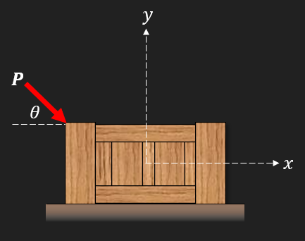
A worker pushes a box of mass \(m\) across a horizontal floor by leaning on it from above with a force \(P\) inclined at an angle \(\theta\) below horizontal, as shown in Figure 7.2.1. The contact between box and floor is governed by kinetic friction with coefficient \(\mu_k\). The push is applied for a short time \(t_p\) and then released, after which the box glides until friction brings it to rest.
We want to answer three questions:
What acceleration does a given push produce?
How fast is the box moving the instant the push ends?
How far does it travel before it stops, and at what time?
Figure 7.2.1
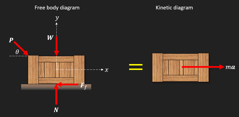
Step 1 - Free body diagram
We isolate the box and mark every force acting on it (Figure 7.2.2). Four forces are present: the inclined push \(\bm F_{\text{ext}}\), the weight \(\bm F_W\) acting downward at the center of mass, the normal force \(\bm F_N\) from the floor acting upward, and the kinetic friction force \(\bm F_f\) acting backward along the direction of motion. With the \(x\)-axis pointing in the direction of motion and \(y\) pointing up, the four force vectors read
The minus signs in \(\bm F_{\text{ext}}\) and \(\bm F_f\) are not arbitrary: the push has a downward component because \(\theta\) measures the inclination below horizontal, and friction opposes the motion which we have taken to be in the \(+x\) direction. The acceleration of the box is purely horizontal,
\[
\bm a = \begin{bmatrix}a_x\\0\end{bmatrix},
\]
since the box stays on the floor.
Figure 7.2.2
Code
mu_k, m, g, P, theta, N, a_x, t = sp.symbols('mu_k m g P theta N a_x t', real=True)FF_ext = P * sp.Matrix([sp.cos(theta), -sp.sin(theta)])FF_N = sp.Matrix([0, N])FF_W = sp.Matrix([0, -m*g])FF_f = sp.Matrix([-mu_k*N, 0])aa = sp.Matrix([a_x, 0])ltx(r"\bm F_{\text{ext}} =", FF_ext,r",\quad \bm F_N =", FF_N,r",\quad \bm F_W =", FF_W,r",\quad \bm F_f =", FF_f)
\[ \bm F_{\text{ext}} =\left[\begin{matrix}P \cos{\left(\theta \right)}\\- P \sin{\left(\theta \right)}\end{matrix}\right],\quad \bm F_N =\left[\begin{matrix}0\\N\end{matrix}\right],\quad \bm F_W =\left[\begin{matrix}0\\- g m\end{matrix}\right],\quad \bm F_f =\left[\begin{matrix}- N \mu_{k}\\0\end{matrix}\right] \]
Step 2 - Equations of motion
Newton’s second law collects the four force vectors on the left and the inertial term on the right,
Written out component by component this is a \(2\times 2\) algebraic system in the two unknowns \(a_x\) and \(N\) (the push \(P\) and the geometric and material parameters are inputs, not unknowns).
Code
eom = sp.Eq(FF_ext + FF_N + FF_W + FF_f, m*aa)ltx(r"\sum \bm F = m\bm a \;\Rightarrow\;", eom.lhs, "=", eom.rhs)
\[ \sum \bm F = m\bm a \;\Rightarrow\;\left[\begin{matrix}- N \mu_{k} + P \cos{\left(\theta \right)}\\N - P \sin{\left(\theta \right)} - g m\end{matrix}\right]=\left[\begin{matrix}a_{x} m\\0\end{matrix}\right] \]
Step 3 - Solve for the acceleration and the normal force
Two scalar equations in two unknowns are solved at once.
\[ \begin{aligned}N &=P \sin{\left(\theta \right)} + g m\\ a_x &=\dfrac{- P \mu_{k} \sin{\left(\theta \right)} + P \cos{\left(\theta \right)} - g m \mu_{k}}{m}\end{aligned} \]
The structure of the result is worth pausing on. The normal force \(N = mg + P\sin\theta\) is larger than the weight alone, because the downward component of the push presses the box harder into the floor. That extra normal force in turn increases the friction force \(\mu_k N\), so the inclined push is less efficient at accelerating the box than a purely horizontal push of the same magnitude. The horizontal component \(P\cos\theta\) does the useful work of accelerating the box; the vertical component \(P\sin\theta\) is wasted twice over, contributing nothing to acceleration and adding to the friction it must overcome. We see this trade-off clearly in the symbolic expression for \(a_x\) before any numbers are inserted, which is exactly why we solve symbolically first.
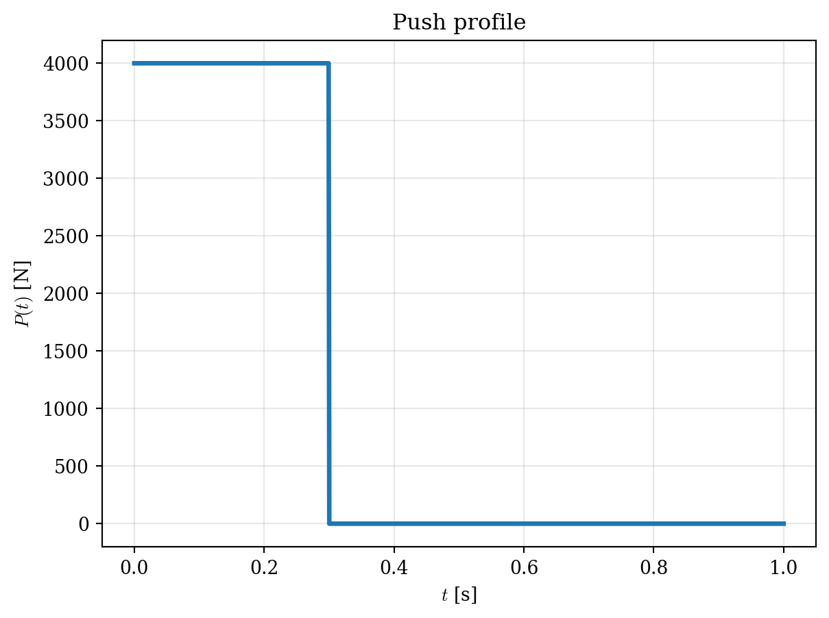
Step 4 - The push profile and the equation of motion in time
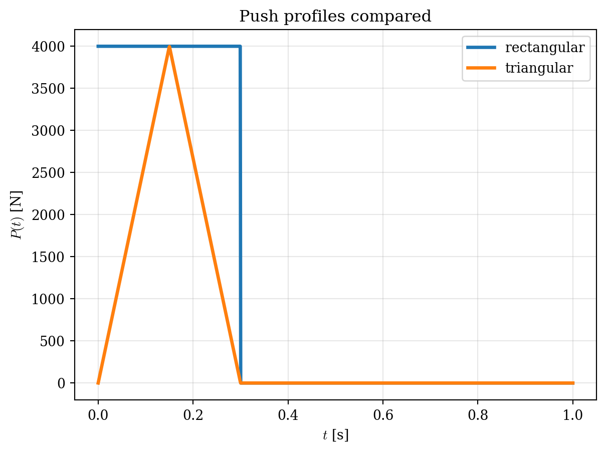
To get a trajectory we have to say how \(P\) depends on time. The simplest model treats the push as a constant force \(P_0\) applied for a short interval \(0 \le t \le t_p\) and zero thereafter,
\[
P(t) = \begin{cases} P_0 & t \le t_p\\ 0 & t > t_p \end{cases}
\]
This piecewise definition splits the motion into two phases: a push phase during which the box accelerates, and a glide phase during which only friction acts and the box decelerates until it stops. We write the equation of motion in the form
\[
\ddot x(t) = a_x\bigl(P(t)\bigr),
\]
substitute the symbolic expression for \(a_x\) obtained above, and solve the resulting ODE phase by phase, matching position and velocity at the boundary \(t = t_p\).
⚠ Note
The friction model we use, \(\bm F_f = -\mu_k N\,\hat{\bm v}\), where \(\hat{\bm v} = \bm v / \|\bm v\|\) is the unit vector along the velocity, is only valid while the box is moving. Once the box comes to rest the kinetic friction model breaks down and we should switch to static friction. We therefore solve until the velocity reaches zero and stop there: any prediction of the box reversing direction would be an artefact of the model, not physics.
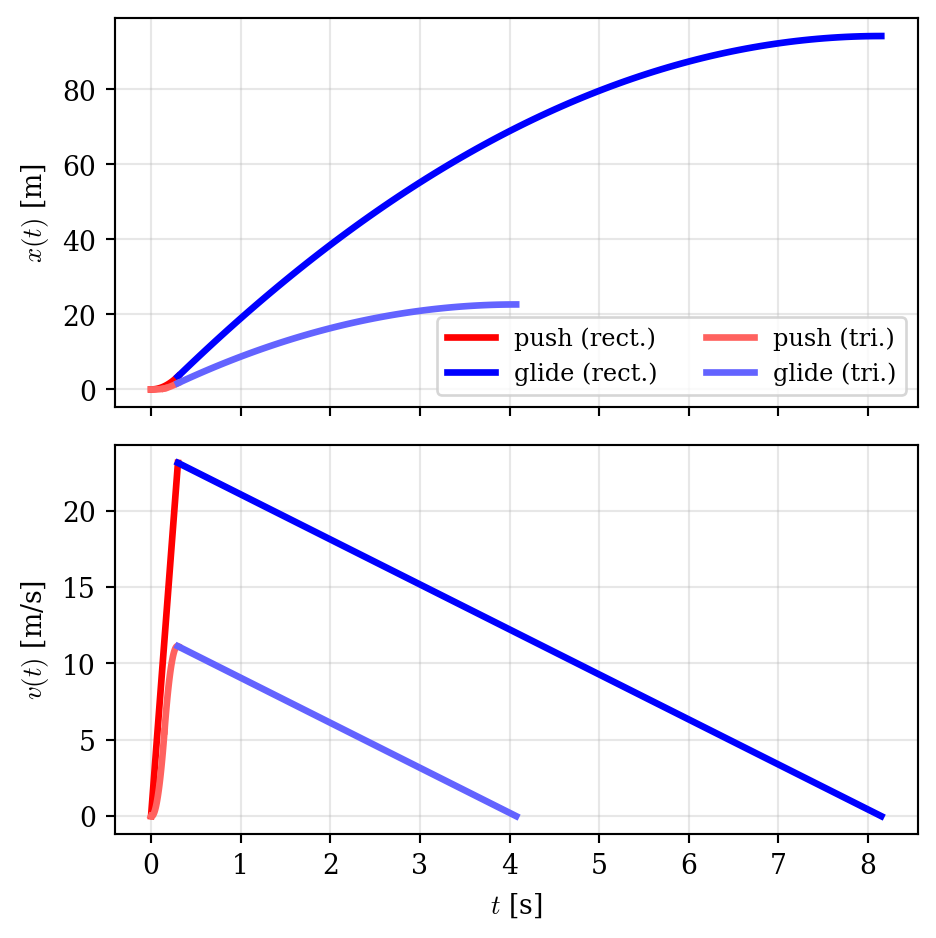
We pick concrete values to make the trajectory visible. A box of \(m = 50\) kg is pushed horizontally (\(\theta = 0\)) with \(P_0 = 4000\) N for \(t_p = 0.3\) s on a floor with \(\mu_k = 0.3\), taking \(g = 9.82\) m/s².
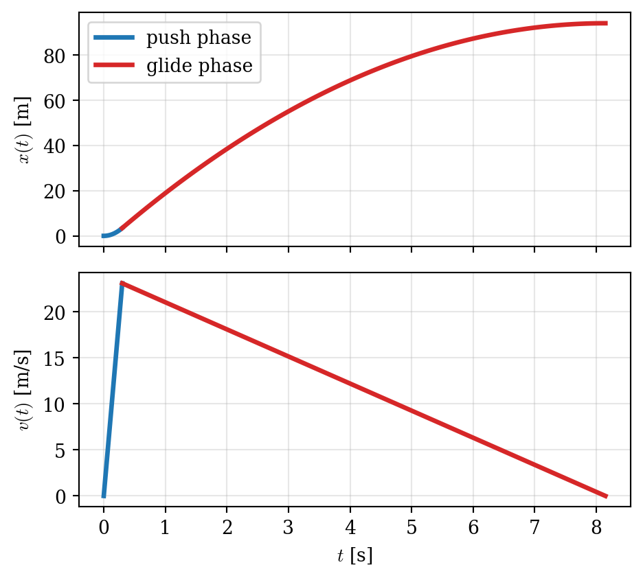
During the push the acceleration is constant and given by \(a_x\) evaluated at \(P = P_0\). The box starts from rest, \(x(0) = 0\) and \(\dot x(0) = 0\), so a single integration gives the velocity and a second gives the position.
The position grows quadratically and the velocity linearly, exactly as we expect for constant acceleration. At the moment the push ends, \(t = t_p\), the box has reached
After the push is released only friction acts on the box, and the acceleration is the negative constant \(-\mu_k g\) (the only horizontal force is friction, since \(N = mg\) once \(P = 0\)). The initial conditions for this phase come from where the push phase ended: position \(x_1(t_p)\) and velocity \(v_1(t_p)\).
The box stops when \(v_2(t) = 0\). Solving this single linear equation for \(t\) gives the stop time, and substituting into \(x_2\) gives the total distance travelled.
The box travels for several seconds and covers tens of meters, almost all of it during the glide phase. The push phase contributes only a small fraction of the total distance, but it sets the velocity that the glide must dissipate.
Step 7 - Visualizing the motion
Plotting position and velocity over the full motion makes the two-phase structure visible at a glance. The kink in the velocity at \(t = t_p\) marks the transition from acceleration to deceleration, and the velocity curve hits zero exactly where the position curve flattens out.
A variant: how does the answer change if we model the push more carefully?
Treating the push as a perfect rectangle in time is a coarse model. A more realistic profile has the force ramp up, peak, and ramp back down over the same total duration \(t_p\). We can capture this with a triangular pulse,
\[
P(t) = \begin{cases}
2P_0\,t/t_p & 0 \le t < t_p/2\\
2P_0\,(t_p - t)/t_p & t_p/2 \le t \le t_p\\
0 & t > t_p
\end{cases}
\]
The peak value is the same \(P_0\) as before but the impulse delivered to the box, \(\int P\,dt\), is exactly half. We expect the box to leave the push phase at a lower velocity and to stop sooner.
Code
P_tri = sp.Piecewise( (2*P0*t/t_p, t < t_p/2), (2*P0*(t_p - t)/t_p, t <= t_p), (0, True),)ltx(r"P_{\triangle}(t) =", P_tri)
Collecting the work from each phase, the full motion under the triangular push is described by three pieces. The acceleration follows the shape of the load: it rises linearly during phase A, falls linearly through zero during phase B, then jumps to the constant friction-only deceleration during the glide. Velocity and position are the running integrals, joined continuously across the phase boundaries by the matching conditions we used to set up the ODEs.
Code
from IPython.display import displaya_A_expr = a_x_sym.subs(vals).subs(P, 2*P0*t/t_p)a_B_expr = a_x_sym.subs(vals).subs(P, 2*P0*(t_p - t)/t_p)x_tri_pw = sp.Piecewise( (x_A, t <= (t_p/2).evalf(4)), (x_B, t <= t_p.evalf(4)), (x_C_tri, t <= t_end_tri.evalf(4)), (x_end_tri, True),)v_tri_pw = sp.Piecewise( (v_A, t <= (t_p/2).evalf(4)), (v_B, t <= t_p.evalf(4)), (v_C_tri, t <= t_end_tri.evalf(4)), (0, True),)a_tri_pw = sp.Piecewise( (a_A_expr, t <= (t_p/2).evalf(4)), (a_B_expr, t <= t_p.evalf(4)), (a2, t <= t_end_tri.evalf(4)), (0, True),)display(ltx(r"\ddot x_\triangle(t) =", a_tri_pw.evalf(4)))display(ltx(r"\dot x_\triangle(t) =", v_tri_pw.evalf(4)))display(ltx(r"x_\triangle(t) =", x_tri_pw.evalf(4)))
\[ \ddot x_\triangle(t) =\begin{cases} 533.3 t - 2.946 & \text{for}\: t \leq 0.15 \\157.1 - 533.3 t & \text{for}\: t \leq 0.3 \\-2.946 & \text{for}\: t \leq 4.073 \\0 & \text{otherwise} \end{cases} \]
\[ \dot x_\triangle(t) =\begin{cases} 0.0006667 t \left(4.0 \cdot 10^{5} t - 4419.0\right) & \text{for}\: t \leq 0.15 \\- 266.7 t^{2} + 157.1 t - 12.0 & \text{for}\: t \leq 0.3 \\12.0 - 2.946 t & \text{for}\: t \leq 4.073 \\0 & \text{otherwise} \end{cases} \]
\[ x_\triangle(t) =\begin{cases} 0.0001111 t^{2} \left(8.0 \cdot 10^{5} t - 1.326 \cdot 10^{4}\right) & \text{for}\: t \leq 0.15 \\- 88.89 t^{3} + 78.53 t^{2} - 12.0 t + 0.6 & \text{for}\: t \leq 0.3 \\- 1.473 t^{2} + 12.0 t - 1.8 & \text{for}\: t \leq 4.073 \\22.64 & \text{otherwise} \end{cases} \]
The triangular pulse delivers half the impulse of the rectangle, and the box ends up traveling roughly a quarter of the distance: the kinetic energy at the end of the push scales as the square of the exit velocity, which itself scales linearly with impulse. This sensitivity to the shape of the load profile is a recurring theme. When the loading is short and intense, the integrated quantity that matters is the impulse, and modelling decisions about exactly how the load rises and falls have a direct impact on the predicted motion.
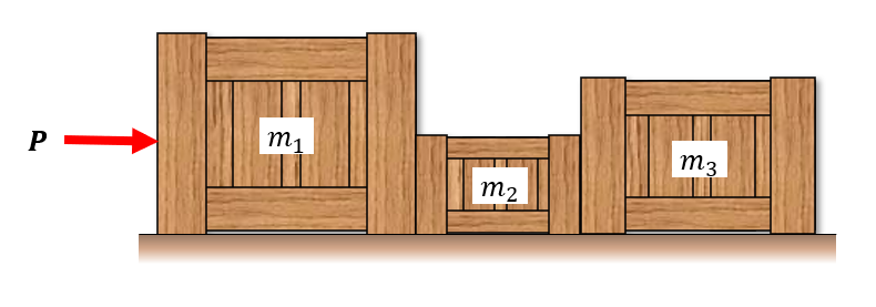
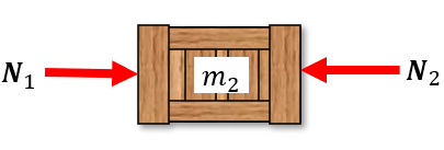
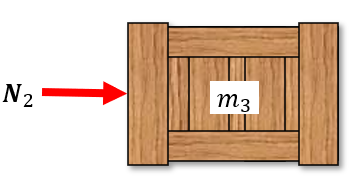
Example 2: Contact forces in a train of boxes
Three boxes of masses \(m_1\), \(m_2\), \(m_3\) rest in a row on a smooth floor, touching one another, and are pushed from behind by a horizontal force \(P\) applied to box 1 (Figure 7.2.3). The floor is frictionless. We want the acceleration of the train and the two internal contact forces between neighbouring boxes.
Figure 7.2.3
Newton II applied to the three boxes as a single body gives the acceleration immediately, \(P = (m_1 + m_2 + m_3)\,a\), but it tells us nothing about the internal contact forces \(N_1\) between boxes 1 and 2 and \(N_2\) between boxes 2 and 3. Internal forces cancel in pairs at the level of the whole system, so to recover them we have to isolate each box on its own and apply Newton’s third law at each contact.
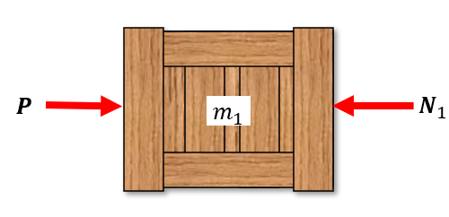
Step 1 - Free body diagrams
We split the system into three free bodies, one per box. At each contact the force exerted on the box ahead is equal in magnitude and opposite in sign to the force exerted on the box behind (Newton’s third law), so the same scalars \(N_1\) and \(N_2\) appear with opposite signs in adjacent equations.
Box 1
Box 2
Box 3
Box 1 is pushed forward by \(P\) and pushed backward by box 2 with magnitude \(N_1\). Box 2 is pushed forward by \(N_1\) and pushed backward by \(N_2\). Box 3 is pushed forward by \(N_2\) alone, since nothing else touches it from behind. Gravity and the normal reaction from the floor balance vertically on each box and have no horizontal component, so they drop out of the equations of motion.
Step 2 - Equations of motion
The horizontal component of \(\bm F = m\bm a\) for each box gives a system of three scalar equations,
These three equations alone contain five unknowns (\(a_1\), \(a_2\), \(a_3\), \(N_1\), \(N_2\)), so the system is not yet solvable. The two missing relations come from kinematics, not kinetics.
Because the boxes remain in contact and the contact is rigid, the three boxes share a single acceleration: \(a_1 = a_2 = a_3 \equiv a\). Substituting this constraint reduces the three equations to a \(3\times 3\) linear system in the unknowns \((a, N_1, N_2)\), which we can solve symbolically.
The acceleration is the one we’d get from treating the train as a single body of total mass \(m_\text{tot} = m_1 + m_2 + m_3\), namely \(a = P/m_\text{tot}\). The internal contact forces have no effect on the centre-of-mass motion, as expected.
\(N_1 = P\,(m_2 + m_3)/m_\text{tot}\) is the force needed to accelerate everything downstream of the first contact, i.e., boxes 2 and 3.
\(N_2 = P\,m_3/m_\text{tot}\) is the force needed to accelerate everything downstream of the second contact, i.e., box 3 alone.
In words: each internal contact carries an amount of force proportional to the mass it has to drag along. The contact closest to the push always carries the largest internal load. This is the same reason the rear coupling on a train of carriages pulls harder than the couplings further forward.
A numerical check
Take \(m_1 = 3\) kg, \(m_2 = 1\) kg, \(m_3 = 2\) kg and \(P = 120\) N. The total mass is \(m_\text{tot} = 6\) kg and the system accelerates at \(a = 20\) m/s². The first contact must accelerate \(m_2 + m_3 = 3\) kg at this rate, giving \(N_1 = 60\) N; the second contact must accelerate \(m_3 = 2\) kg, giving \(N_2 = 40\) N.
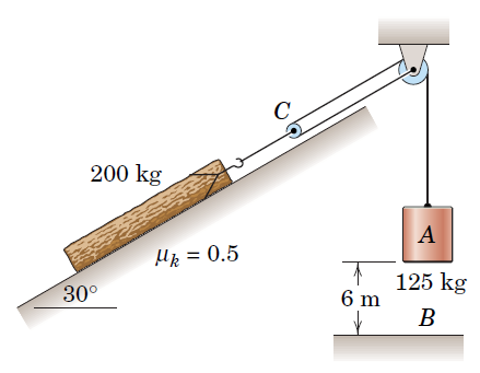
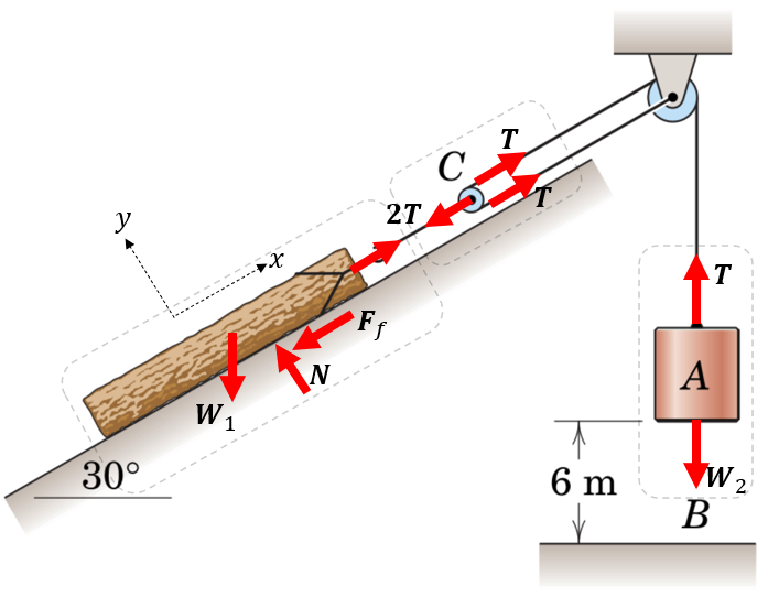
Example 3: A log on a ramp, pulled by a pulley system
A log of mass \(m_1\) rests on a ramp inclined at angle \(\theta\) with kinetic friction coefficient \(\mu_k\). A rope wraps around a pulley attached to the log and runs over a fixed pulley to a counterweight of mass \(m_2\) (Figure 7.2.4). The counterweight is released from rest and falls a distance \(h\) to the ground. We want its velocity at impact.
Figure 7.2.4
The pulley arrangement is what makes this problem more than a free fall with a brake. Two rope segments connect to the log while only one connects to the counterweight, giving a 2:1 mechanical advantage: the log feels twice the rope tension but moves only half as far as the counterweight.
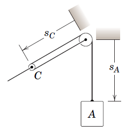
Step 1 - The kinematic constraint
Let \(s_C\) measure the log’s position up the ramp and \(s_A\) the counterweight’s position downward from its starting point, both positive in the direction the system actually moves. The rope is inextensible, so its total length is constant. From Figure 7.2.5 this length is
\[
L = 2\,s_C + s_A.
\]
Differentiating twice in time gives the acceleration constraint
\[
a_A = 2\,a_C,
\]
which says that for every metre the log climbs, the counterweight falls two metres.
Figure 7.2.5
Step 2 - Free body diagrams
We isolate the log and the counterweight (Figure 7.2.6). On the log the rope tension contributes \(2T\) up the ramp, since the log’s pulley is held by two rope segments each carrying tension \(T\). On the counterweight only one rope segment acts, contributing \(T\) upward. This is the kinetic mirror of the kinematic 2:1: the rope trades tension for displacement.
Figure 7.2.6
Step 3 - Equations of motion
Newton’s second law for the log along the ramp (positive up) and perpendicular to it gives
\[
\begin{aligned}
2T - m_1 g \sin\theta - \mu_k N &= m_1\,a_C\\
N - m_1 g \cos\theta &= 0.
\end{aligned}
\]
For the counterweight, with positive \(s_A\) pointing down, only weight and tension act:
\[
m_2 g - T = m_2\,a_A.
\]
Together with the kinematic constraint \(a_A = 2 a_C\), this is four equations in the four unknowns \((T, N, a_C, a_A)\).
Code
m1, m2, theta_s, mu_k_s, g_s, T, N_s, aC, aA = sp.symbols('m_1 m_2 theta mu_k g T N a_C a_A', real=True, positive=True)eom_log_x = sp.Eq(2*T - m1*g_s*sp.sin(theta_s) - mu_k_s*N_s, m1*aC)eom_log_y = sp.Eq(N_s - m1*g_s*sp.cos(theta_s), 0)eom_counter = sp.Eq(m2*g_s - T, m2*aA)constraint = sp.Eq(aA, 2*aC)eqs = [eom_log_x, eom_log_y, eom_counter, constraint]eqs | la
\[ {\def\arraystretch{1.0}\begin{bmatrix}
- N \mu_{k} + 2 T - g m_{1} \sin{\left(\theta \right)} = a_{C} m_{1} \\
N - g m_{1} \cos{\left(\theta \right)} = 0 \\
- T + g m_{2} = a_{A} m_{2} \\
a_{A} = 2 a_{C}
\end{bmatrix}} \]
The numerator of \(a_C\) is the net pull on the system: the counterweight contributes \(2 m_2 g\) (twice its weight, because the pulley doubles its displacement) while the log’s weight and friction resist with \(m_1 g \sin\theta + \mu_k m_1 g \cos\theta\). If the numerator goes negative, kinetic friction does not apply at all: static friction holds the log in place and the counterweight cannot move. We assume the geometry guarantees motion.
The denominator \(m_1 + 4 m_2\) is the system’s effective inertia viewed from the log. Any kinetic energy stored in the moving system can be written as \(\tfrac{1}{2}(m_1 + 4 m_2) v_C^2\) once the constraint \(v_A = 2 v_C\) is used: the counterweight enters as \(4 m_2\) because it moves twice as fast, and kinetic energy goes as the square of velocity.
\[ \begin{aligned}N &=1699.0\;\text{N}\\ T &=1004.0\;\text{N}\\ a_C &=0.8885\;\text{m/s}^2\\ a_A &=1.777\;\text{m/s}^2\end{aligned} \]
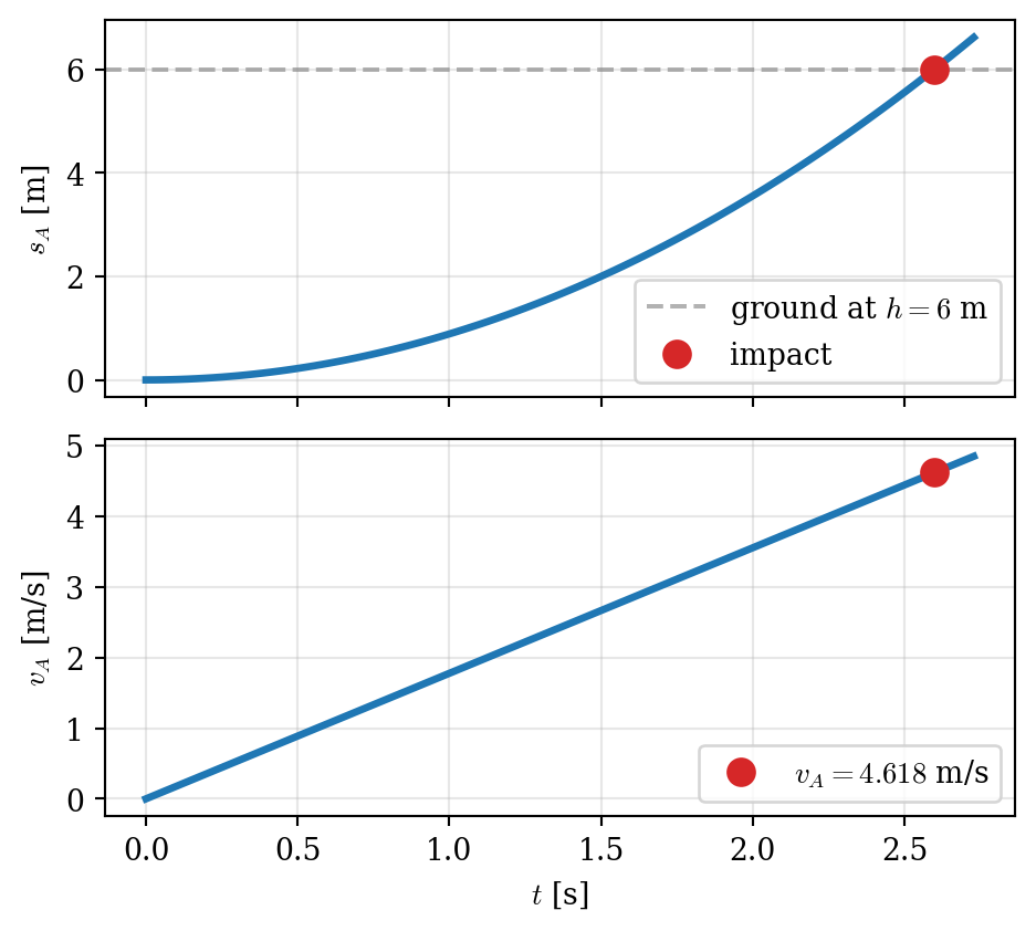
Step 5 - Velocity at impact
The question we are asking, how fast is the counterweight moving when it has fallen \(h\)?, depends on position rather than time, so it pays to integrate over distance instead of integrating in time. We start with the differential relation
\[
a_A\,ds_A \;=\; v_A\,dv_A,
\]
which is established in 6.3.3. Integrating both sides, from rest at \(s_A = 0\) to the impact velocity at \(s_A = h\),
reduces the problem to two simple antiderivatives. Since \(a_A\) is constant, the left side is \(a_A h\); the right side is \(v_A^2/2\). Solving for \(v_A\) gives the impact velocity directly, without ever computing \(s_A(t)\) or \(v_A(t)\) as functions of time.
The method above sidesteps time by integrating over distance, which is a direct route when only the impact velocity is wanted. But we can of course just solve the differential equation \(\ddot s_A = a_A\) and get full expressions for the position and velocity as functions of time. Two integrations against the initial conditions \(s_A(0) = 0\), \(\dot s_A(0) = 0\) are all it takes; we hand the ODE to sympy’s dsolve. Once \(s_A(t)\) is in hand we set \(s_A(t_{\text{impact}}) = h\), solve for the impact time, and read off \(v_A\) at that instant.
Setting \(s_A(t) = h\) gives a quadratic in \(t\),
\[
\tfrac{1}{2} a_A\,t^2 = h
\quad\Longrightarrow\quad
t = \pm\sqrt{\frac{2 h}{a_A}}.
\]
Both roots are real but only the positive one is physical: the negative root corresponds to the time before release at which a body decelerating to rest would have been at the ground, which is meaningless here. We pick the positive root and substitute it into \(v_A(t)\) to get the impact velocity.
Code
sA_num = sA_t.subs(vals3)roots = sp.solve(sp.Eq(sA_num, h), t)display(ltx(r"\text{roots of } s_A(t) - h = 0:\quad t \in", sp.FiniteSet(*roots)))t_impact =next(r for r in roots if r.is_real and r >0)v_impact = vA_t.subs(vals3).subs(t, t_impact)display(ltx(r"t_{\text{impact}} &=", t_impact, r"\approx", t_impact.evalf(4), r"\;\text{s}",r"\\ v_A(t_{\text{impact}}) &=", v_impact, r"\approx", v_impact.evalf(4), r"\;\text{m/s}", aligned=True))
\[ \text{roots of } s_A(t) - h = 0:\quad t \in\left\{- \dfrac{20 \sqrt{2289}}{327 \sqrt{3 - \sqrt{3}}}, \dfrac{20 \sqrt{2289}}{327 \sqrt{3 - \sqrt{3}}}\right\} \]
Plotting position and velocity over the fall makes the impact instant easy to read off: the position curve hits the ground line \(s_A = h\) at \(t_{\text{impact}}\), and the velocity curve crosses that vertical at the impact velocity.