6.2  Forward kinematics

The problem

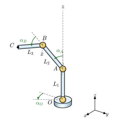
The arm in Figure 6.2.1 has three links \(OA\), \(AB\) and \(BC\) of lengths \(L_1\), \(L_2\) and \(L_3\). The joint at \(O\) turns the whole arm about the global \(z\) axis through the angle \(\alpha_O\). The joints at \(A\) and \(B\) turn about the axis \(\tilde x\), perpendicular to the plane of the arm, through \(\alpha_A\) and \(\alpha_B\), each measured from the line of the previous link. With all three angles zero the arm stands straight up along \(z\).

Determine the position \(\bm r_{OC}\) of the end effector as a function of the three joint angles, and evaluate it for \(L_1 = L_2 = L_3 = 1\), \(\alpha_O = 0\) and \(\alpha_A = \alpha_B = 45^\circ\).

Frames that travel with the links

Each link is simplest to describe in a frame attached to it, in which it points along the local \(z\) axis. In its own frame every link vector is a length times \(\bm e_z\),

\[ \bm r'_{OA} = L_1 \bm e_z, \qquad \bm r'_{AB} = L_2 \bm e_z, \qquad \bm r'_{BC} = L_3 \bm e_z, \qquad \bm e_z = [0, 0, 1]^\mathsf{T} \tag{6.2.1}\]

where the prime marks components in the local frame. A frame is described by a rotation matrix \(\bm R\) whose three columns are its basis vectors written in global components. A vector with local components \(\bm v'\) therefore has the global components \(\bm v = \bm R \bm v'\), since \(\bm R \bm v'\) is the sum of the basis vectors weighted by the local components. The global frame itself is the identity matrix.

The joints turn about coordinate axes, and the right-hand rule fixes the sign. A positive rotation through \(\alpha\) about \(z\) and about \(x\) is

\[ \bm R_z(\alpha) = \begin{bmatrix} \cos\alpha & -\sin\alpha & 0 \\ \sin\alpha & \cos\alpha & 0 \\ 0 & 0 & 1 \end{bmatrix}, \qquad \bm R_x(\alpha) = \begin{bmatrix} 1 & 0 & 0 \\ 0 & \cos\alpha & -\sin\alpha \\ 0 & \sin\alpha & \cos\alpha \end{bmatrix}. \tag{6.2.2}\]

The base joint turns about the global \(z\) axis, so the frame of the first link is \(\bm R_1 = \bm R_z(\alpha_O)\).

The joint at \(A\) turns about the \(x\) axis of frame 1, \(\tilde{\bm x} = \bm R_1 \bm e_x\), which coincides with the global \(x\) axis only when \(\alpha_O = 0\). A rotation about this carried axis is done in three steps: express the vector in frame 1 with \(\bm R_1^\mathsf{T}\), rotate it about the local \(x\) axis with \(\bm R_x\), and return to global components with \(\bm R_1\),

\[ \bm R_{\tilde x}(\alpha_A) = \bm R_1 \bm R_x(\alpha_A) \bm R_1^\mathsf{T}. \]

Applying this rotation to the frame \(\bm R_1\) gives the frame of the second link,

\[ \bm R_2 = \bm R_{\tilde x}(\alpha_A)\, \bm R_1 = \bm R_1 \bm R_x(\alpha_A) \bm R_1^\mathsf{T} \bm R_1 = \bm R_1 \bm R_x(\alpha_A) \]

because \(\bm R_1^\mathsf{T} \bm R_1 = \bm I\) for a rotation matrix. A rotation about an axis that moves with the arm multiplies the frame from the right, with the elementary matrix of 6.2.2, while a rotation about a fixed global axis multiplies from the left. The joint at \(B\) turns about the \(x\) axis of frame 2, which is the same axis \(\tilde{\bm x}\) since \(\bm R_x\) leaves the \(x\) axis in place, and the same argument gives \(\bm R_3 = \bm R_2 \bm R_x(\alpha_B)\).

Each link vector in global components is its frame times its local vector, and the end effector is reached by adding the links from the base,

\[ \boxed{ \begin{aligned} \bm R_1 &= \bm R_z(\alpha_O), \qquad \bm R_2 = \bm R_1 \bm R_x(\alpha_A), \qquad \bm R_3 = \bm R_2 \bm R_x(\alpha_B) \\ \bm r_{OC} &= \bm R_1 \bm r'_{OA} + \bm R_2 \bm r'_{AB} + \bm R_3 \bm r'_{BC} \end{aligned} } \tag{6.2.3}\]

The pattern extends to any number of links. Link \(k\) has the frame \(\bm R_k = \bm R_{k-1} \bm R_{a_k}(\alpha_k)\), where \(a_k\) is the local axis of its joint, and the position of its far end is the sum of \(\bm R_j \bm r'_j\) over the links from the base up to \(k\).

Implementation

6.2.3 translates line by line. SymPy’s rot_ccw_axis3 and rot_ccw_axis1 are \(\bm R_z\) and \(\bm R_x\) of 6.2.2, positive by the right-hand rule, and the @ operator is the matrix product.

alpha_O, alpha_A, alpha_B = sp.symbols('alpha_O alpha_A alpha_B', real=True)
L_1, L_2, L_3 = sp.symbols('L_1 L_2 L_3', positive=True)
e_z = sp.Matrix([0, 0, 1])

R_1 = sp.rot_ccw_axis3(alpha_O)              # the base joint turns about global z
R_2 = R_1 @ sp.rot_ccw_axis1(alpha_A)        # joint A turns about the carried x axis
R_3 = R_2 @ sp.rot_ccw_axis1(alpha_B)        # joint B turns about the same carried axis

rr_OA = R_1 @ (L_1*e_z)                      # each link: its frame times its local vector
rr_AB = R_2 @ (L_2*e_z)
rr_BC = R_3 @ (L_3*e_z)
rr_OC = sp.simplify(rr_OA + rr_AB + rr_BC)

ltx(r"\bm r_{OC} =", rr_OC)

A check by hand

The joints at \(A\) and \(B\) turn about the same axis \(\tilde{\bm x}\), so the three links stay in one plane, the vertical plane through \(z\) perpendicular to \(\tilde{\bm x}\). Inside frame 1 the arm is a planar two-link arm standing on a post of height \(L_1\). A link at the angle \(\alpha\) from the vertical points along \(\bm R_x(\alpha)\bm e_z = [0, -\sin\alpha, \cos\alpha]^\mathsf{T}\), and the angles add along the chain because \(\bm R_x(\alpha_A)\bm R_x(\alpha_B) = \bm R_x(\alpha_A + \alpha_B)\). The horizontal reach of the tip and its height are then

\[ \rho = L_2 \sin\alpha_A + L_3 \sin(\alpha_A + \alpha_B), \qquad z_C = L_1 + L_2 \cos\alpha_A + L_3 \cos(\alpha_A + \alpha_B) \]

and the reach points along \(-\bm e_y\) in frame 1. The base joint turns that direction to \(\bm R_z(\alpha_O)(-\bm e_y) = [\sin\alpha_O, -\cos\alpha_O, 0]^\mathsf{T}\), which gives

\[ \bm r_{OC} = \begin{bmatrix} \rho \sin\alpha_O \\ -\rho\cos\alpha_O \\ z_C \end{bmatrix}. \tag{6.2.4}\]

The difference between the two results should vanish identically.

rho = L_2*sp.sin(alpha_A) + L_3*sp.sin(alpha_A + alpha_B)
z_C = L_1 + L_2*sp.cos(alpha_A) + L_3*sp.cos(alpha_A + alpha_B)
rr_OC_hand = sp.Matrix([rho*sp.sin(alpha_O), -rho*sp.cos(alpha_O), z_C])

ltx(r"\bm r_{OC} - \bm r_{OC}^{\text{hand}} =", sp.simplify(rr_OC - rr_OC_hand))

The chain of frames and the planar argument agree. The planar argument is the shorter one here, but it depends on two joint axes being parallel, and it has no counterpart for a wrist whose three axes point in three directions. 6.2.3 works for any arrangement.

Numbers and a picture

With unit links, \(\alpha_O = 0\) and \(\alpha_A = \alpha_B = 45^\circ\), 6.2.4 gives \(\rho = \sin 45^\circ + \sin 90^\circ\) and \(z_C = 1 + \cos 45^\circ + \cos 90^\circ\), so the reach and the height are both \(1 + \sqrt 2/2\).

vals = {L_1: 1, L_2: 1, L_3: 1, alpha_O: 0, alpha_A: sp.pi/4, alpha_B: sp.pi/4}
ltx(r"\bm r_{OC} =", rr_OC.subs(vals).evalf(4))

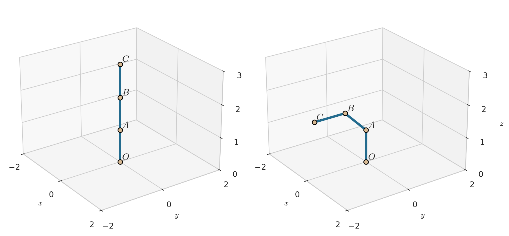
The tip lies at \(y = -1.707\) and \(z = 1.707\) in units of the link length. Figure 6.2.2 draws the arm in the straight configuration and in this one, from the three link vectors of the code. With \(\alpha_O = 0\) the bent arm lies in the plane \(x = 0\) and leans toward negative \(y\), as 6.2.4 predicts.

Code

links = sp.lambdify([alpha_O, alpha_A, alpha_B],
                    [v.subs({L_1: 1, L_2: 1, L_3: 1}) for v in (rr_OA, rr_AB, rr_BC)])

fig = plt.figure(figsize=(9, 4.5))
for k, angles in enumerate([(0, 0, 0), (0, np.pi/4, np.pi/4)]):
    ax = fig.add_subplot(1, 2, k + 1, projection='3d')
    points = np.cumsum([np.zeros(3)] + [np.ravel(v) for v in links(*angles)], axis=0)
    ax.plot(*points.T, color='#236B8E', lw=3, marker='o', ms=6, mfc='#d8ba94', mec='k')
    for p, name in zip(points, 'OABC'):
        ax.text(*(p + [0.1, 0, 0.1]), f'${name}$', fontsize=12)
    ax.set(xlim=(-2, 2), ylim=(-2, 2), zlim=(0, 3), xticks=[-2, 0, 2], yticks=[-2, 0, 2],
           zticks=[0, 1, 2, 3], xlabel='$x$', ylabel='$y$', zlabel='$z$')
    ax.set_box_aspect((4, 4, 3))
    ax.view_init(elev=25, azim=-35)
plt.tight_layout()
plt.show()

Velocity and singular configurations

When the motors turn, the joint angles change with time and the tip moves. Differentiating 6.2.3 with the chain rule gives the velocity of the tip as a linear combination of the joint rates,

\[ \begin{aligned} \dot{\bm r}_{OC} &= \bm J \dot{\bm\alpha} \\ \bm J &= \frac{\partial \bm r_{OC}}{\partial \bm\alpha} = \begin{bmatrix} \dfrac{\partial \bm r_{OC}}{\partial \alpha_O} & \dfrac{\partial \bm r_{OC}}{\partial \alpha_A} & \dfrac{\partial \bm r_{OC}}{\partial \alpha_B} \end{bmatrix} \\ \bm\alpha &= [\alpha_O, \alpha_A, \alpha_B]^\mathsf{T} \end{aligned} \tag{6.2.5}\]

where the \(3 \times 3\) matrix \(\bm J\) is the Jacobian of the arm. Its column \(k\) is the velocity of the tip when joint \(k\) turns at unit rate and the others are held. The base joint, for example, moves the tip on a circle about \(z\), so its column is \(\bm e_z \times \bm r_{OC}\). Inverse kinematics at the level of velocities means solving 6.2.5 for \(\dot{\bm\alpha}\), and that fails where \(\det \bm J = 0\).

J = rr_OC.jacobian([alpha_O, alpha_A, alpha_B])
det_J = sp.factor(sp.simplify(J.det()))
ltx(r"\det \bm J =", det_J.subs(rho, sp.Symbol('rho')))      # rho: the reach of the hand check

Here \(\rho\) is the horizontal reach of the tip from the hand check, and the determinant vanishes in two ways. When \(\rho = 0\) the tip lies on the \(z\) axis, and turning the base joint does not move it at all, so the first column of \(\bm J\) is zero. When \(\sin\alpha_B = 0\) the last two links are in line, stretched or folded back, and no combination of joint rates moves the tip along that line. These are the singular configurations of the arm. Close to them a modest tip velocity demands very large joint rates, and a controller that follows a path through one has to slow down or leave the path. The straight configuration on the left of Figure 6.2.2 is singular in both ways at once, which makes the natural start position the worst place from which to steer the tip.

Interactive example

The marimo notebook below has a slider for each joint angle and draws the arm from 6.2.3 as the sliders move. Moving the tip toward the \(z\) axis, or stretching the last two links into line, shows the singular configurations of 6.2.5 directly.