g, v0, C = 9.81, 20.0, 3.0

def euler_loop(ds):
    x, y, theta, t = [0.0], [0.0], [0.0], [0.0]
    while theta[-1] < 2*np.pi:                       # until the track has turned a full revolution
        v2 = v0**2 - 2*g*y[-1]                       # the speed squared at this height
        theta.append(theta[-1] + C*g/v2*ds)          # the track turns faster where the train is slower
        x.append(x[-1] + np.cos(theta[-1])*ds)
        y.append(y[-1] + np.sin(theta[-1])*ds)
        t.append(t[-1] + ds/np.sqrt(v2))             # time to cover ds at the current speed
    return np.array(x), np.array(y), np.array(theta), np.array(t)

x, y, theta, t = euler_loop(0.5)6.4 Roller coaster loop
“Math has been liberated from calculating. See, I think of calculating as the machinery of math, it’s the mechanism for doing it. But it isn’t an end in itself.”
— Conrad Wolfram, Stop Teaching Calculating, Start Teaching Math, TEDGlobal, 2010
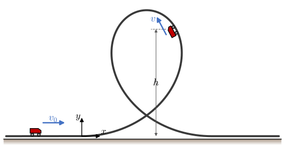
A train enters a loop at speed \(v_0\), and we want the loop shaped so that the normal acceleration of the train stays at a constant multiple \(C\) of \(g\) all the way round. The train slows as it climbs, so the radius of curvature has to shrink with the speed, and the loop grows tall and narrow at the top. Particle kinematics in natural coordinates gives the equations for the shape. They are three coupled differential equations in the arc length, and one of them has no closed-form solution, so we solve them with forward Euler and let the same loop give us the time along the track as well.
The video below explains the physics of real loops.
Problem
Determine the shape of a loop entered at \(v_0 = 20\) m/s whose normal acceleration is constant and equal to \(C g\) with \(C = 3\). Friction and air drag are neglected, and the train is treated as a particle.
Speed and height
With no friction and no drag, the kinetic energy at entry is shared between potential energy and the kinetic energy that remains at the height \(h\),
\[ \frac{1}{2}mv_0^2 = mgh + \frac{1}{2}mv^2 . \]
We measure the height by the coordinate \(y\), so \(h = y\) and
\[ v^2 = v_0^2 - 2gy . \tag{6.4.1}\]
Normal acceleration and the load on the rider
The track makes the angle \(\theta\) with the horizontal, and \(\bm e_n\) points toward the centre of curvature. The forces on the train are its weight and the normal force \(N\) from the track.
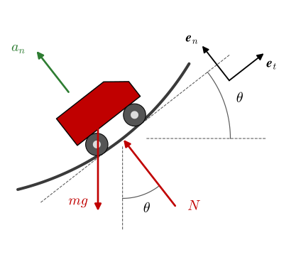
Newton’s second law along \(\bm e_n\) reads
\[ N - mg\cos\theta = m a_n , \]
and the normal acceleration is \(a_n = v^2/R\), from the acceleration in natural coordinates in Particle kinematics. Dividing by \(mg\) gives the normal force in units of the weight,
\[ G := \frac{N}{mg} = \frac{v^2}{gR} + \cos\theta , \]
which is the load the rider feels, often called the g-force. The design condition fixes the first term, \(a_n = v^2/R = Cg\), so the radius of curvature at the height \(y\) follows from 6.4.1,
\[ R = \frac{v^2}{Cg} = \frac{v_0^2 - 2gy}{Cg} , \tag{6.4.2}\]
and the rider feels \(G = C + \cos\theta\). With \(C = 3\) that is \(4\) at the bottom of the loop and \(2\) at the top, where the rider hangs upside down.
The shape from the arc length
We describe the track by its arc length \(s\) from the entry. Over a short arc \(ds\) the track turns through \(d\theta\) about its centre of curvature, and the arc is close to a straight line at the angle \(\theta\) to the horizontal.
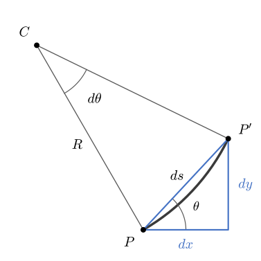
This gives \(ds = R\,d\theta\), \(dx = \cos\theta\,ds\) and \(dy = \sin\theta\,ds\). With 6.4.2 for \(R\), the shape is the solution of
\[ \begin{aligned} \frac{d\theta}{ds} &= \frac{Cg}{v_0^2 - 2gy} , \\ \frac{dx}{ds} &= \cos\theta , \\ \frac{dy}{ds} &= \sin\theta , \end{aligned} \tag{6.4.3}\]
from \(x = y = \theta = 0\) at \(s = 0\) until \(\theta = 2\pi\), when the track is level again and the loop is complete. The turning rate depends on the height and the height on the angle, so the three equations have to be solved together.
Forward Euler
We replace each derivative in 6.4.3 by a forward difference over a step \(\Delta s\) that we choose ourselves. It sets the resolution of the discrete track, much like the time step in Example 6 of Particle kinematics. The angle is updated first, and the new angle moves the point:
\[ \begin{aligned} \theta_{i+1} &= \theta_i + \frac{Cg}{v_0^2 - 2gy_i}\,\Delta s , \\ x_{i+1} &= x_i + \cos\theta_{i+1}\,\Delta s , \\ y_{i+1} &= y_i + \sin\theta_{i+1}\,\Delta s . \end{aligned} \]
The same loop also gives the time. The train covers \(ds = v\,dt\), so \(t_{i+1} = t_i + \Delta s/v_i\) with \(v_i\) from 6.4.1.
Code
fig, ax = plt.subplots(figsize=(6, 5))
ax.plot(x, y, '.-', color='C0', ms=4)
ax.set_aspect('equal')
ax.set_xlabel('$x$ [m]')
ax.set_ylabel('$y$ [m]')
ax.grid(alpha=0.3)
plt.show()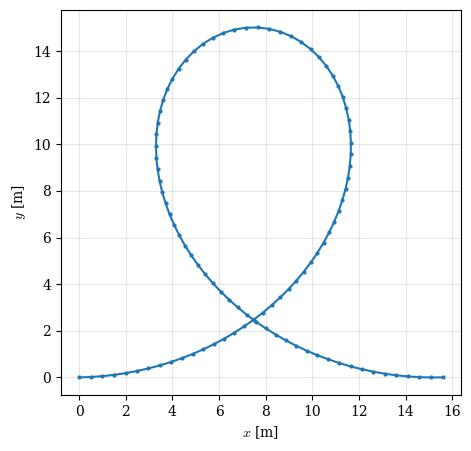
The loop closes on itself where the train leaves it, level at the height it entered, after a ride of about three seconds.
Code
ltx(r"s_{\text{end}} &=", sp.Float(0.5*(len(x) - 1)), r"~\text{m}",
    r"\\ t_{\text{end}} &=", sp.Float(t[-1]), r"~\text{s}",
    r"\\ y_{\max} &=", sp.Float(y.max()), r"~\text{m}", aligned=True, precision=4)
\[ \begin{aligned}s_{\text{end}} &=49.0~\text{m}\\ t_{\text{end}} &=3.152~\text{s}\\ y_{\max} &=15.01~\text{m}\end{aligned} \]
Verification: the height of the loop
The angle and the height can be found exactly, which gives the numerical solution something to be checked against. Dividing the first equation of 6.4.3 by the third removes \(s\), and with \(d(v^2) = -2g\,dy\) from 6.4.1 the variables separate,
\[ \sin\theta\,d\theta = \frac{Cg\,dy}{v^2} = -\frac{C}{2}\,\frac{d(v^2)}{v^2} . \]
We integrate from the entry, where \(\theta = 0\) and \(v = v_0\).
Code
th, phi, w = sp.symbols('theta phi w', real=True)
v_0, g_, C_ = sp.symbols('v_0 g C', positive=True)
v2 = sp.Symbol('v^2', positive=True)

lhs = sp.integrate(sp.sin(phi), (phi, 0, th))
rhs = sp.integrate(-C_/(2*w), (w, v_0**2, v2))
v2_of_theta = sp.powsimp(sp.expand(sp.solve(sp.Eq(lhs, rhs), v2)[0]))
ltx(r"1 - \cos\theta &= ", rhs, r"\\ v^2 &=", v2_of_theta, aligned=True)
\[ \begin{aligned}1 - \cos\theta &= - \dfrac{C \log{\left(v^{2} \right)}}{2} + \dfrac{C \log{\left(v_{0}^{2} \right)}}{2}\\ v^2 &=v_{0}^{2} e^{\dfrac{2 \left(\cos{\left(\theta \right)} - 1\right)}{C}}\end{aligned} \]
6.4.1 turns the speed into the height at every angle, and at the top, \(\theta = \pi\), into the height of the loop.
Code
y_of_theta = (v_0**2 - v2_of_theta)/(2*g_)
y_top = sp.expand(y_of_theta.subs(th, sp.pi)).collect(v_0**2/(2*g_))
y_top_num = y_top.subs({v_0: v0, g_: g, C_: C})
ltx(r"y &=", y_of_theta, r"\\ y_{\text{top}} &=", y_top, r"\\ &=", y_top_num.evalf(6),
    r"~\text{m}", aligned=True)
\[ \begin{aligned}y &=\dfrac{- v_{0}^{2} e^{\dfrac{2 \left(\cos{\left(\theta \right)} - 1\right)}{C}} + v_{0}^{2}}{2 g}\\ y_{\text{top}} &=\dfrac{v_{0}^{2} \left(1 - e^{- \dfrac{4}{C}}\right)}{2 g}\\ &=15.0133~\text{m}\end{aligned} \]
Every Euler station carries its own angle \(\theta_i\), so the exact height at that angle can be compared with \(y_i\) all along the loop. Forward Euler is first-order accurate, and the largest difference should shrink in proportion to \(\Delta s\).
Code
y_exact = sp.lambdify(th, y_of_theta.subs({v_0: v0, g_: g, C_: C}), 'numpy')
steps = np.array([0.5, 0.1, 0.02, 0.004])
errors = []
for ds in steps:
    _, y_i, theta_i, _ = euler_loop(ds)
    errors.append(np.abs(y_i - y_exact(theta_i)).max())

fig, ax = plt.subplots(figsize=(5, 3.5))
ax.loglog(steps, errors, 'o-', label='forward Euler')
ax.loglog(steps, steps/2, 'k--', lw=0.8, label=r'$\Delta s/2$')
ax.set_xlabel(r'$\Delta s$ [m]')
ax.set_ylabel(r'$\max_i |y_i - y(\theta_i)|$ [m]')
ax.legend()
ax.grid(True, which='both', alpha=0.3)
plt.show()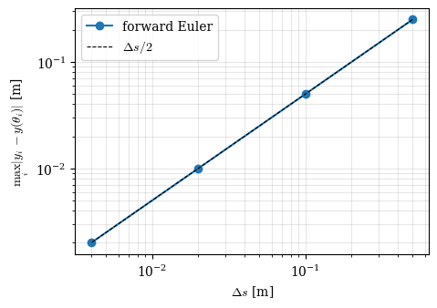
The error falls fivefold with each fivefold smaller step, and with \(\Delta s = 0.5\) m the track is already within 0.25 m of the exact height everywhere.
The top of the loop checks out, but the horizontal position has no such shortcut. Along the track \(dx/d\theta = R\cos\theta = v^2\cos\theta/(Cg)\), which with the speed above is
\[ \frac{dx}{d\theta} = \frac{v_0^2 e^{-2/C}}{Cg}\, e^{a\cos\theta}\cos\theta , \qquad a = \frac{2}{C} . \]
The integral of \(e^{a\cos\theta}\cos\theta\) has no elementary antiderivative, and SymPy returns it unevaluated.
Code
a = sp.Symbol('a', positive=True)
sp.Integral(sp.exp(a*sp.cos(th))*sp.cos(th), th).doit()
\(\displaystyle \int e^{a \cos{\left(\theta \right)}} \cos{\left(\theta \right)}\, d\theta\)
Riding the loop
The accelerations follow from the solution without further work. The normal acceleration is \(Cg\) on the loop by design. The tangential one is the rate of change of the speed, and with \(v\,dv = -g\,dy\) from 6.4.1,
\[ a_t = \frac{dv}{dt} = v\frac{dv}{ds} = -g\frac{dy}{ds} = -g\sin\theta , \]
so the train loses speed at up to \(1g\) on the way up and gains it on the way down. Figure 6.4.4 runs the train through the loop with the time \(t_i\) from the Euler loop, together with \(a_n\), \(a_t\) and the load \(G = C + \cos\theta\) on the rider.
The plot shows a flaw of the design. On the straight track the rider feels \(1g\), and at the entry of the loop the curvature jumps from zero to \(Cg/v_0^2\), so the load jumps to \(4g\) at once, and back again at the exit. A real track eases the curvature in over a transition curve so that the load builds up gradually. The same Euler loop handles that, since only the turning rate \(d\theta/ds\) changes.