“The best modern experiments support the conclusion that Poisson’s ratio can differ sensibly from the value ¼ in materials which may without cavil be treated as isotropic and homogeneous.”
— A. E. H. Love, A Treatise on the Mathematical Theory of Elasticity, 1892
Stress measures how hard the material is being worked. Strain measures how much it has moved as a result. The two are separate ideas, and keeping them separate matters: stress is a statement about force, strain is a statement about geometry, and only a material model links them. This chapter builds the geometric half.
Engineering strain
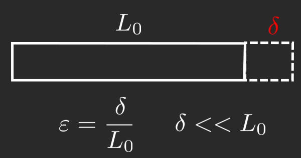
A bar of original length \(L_0\) is stretched to a new length \(L\), as in Figure 8.5.1. The change in length is the deformation\(\delta = L - L_0\), and dividing it by the original length gives the engineering strain, also called the linear strain,
which is dimensionless. Since the numbers involved are usually small, strain is often quoted in percent or in microstrain, where \(1000~\mu\varepsilon\) means \(\varepsilon = 0.001\). Steel yields at roughly \(0.2\%\) strain, so the deformations we work with are genuinely tiny, and that smallness is what makes the linear theory of this book usable.
Figure 8.5.1: A bar of original length \(L_0\) stretched to \(L\), with the deformation \(\delta = L - L_0\).
Figure 8.5.2: Engineering strain is the deformation divided by the original length, which is meaningful only while \(\delta \ll L_0\).
Definition 8.5.1 describes the bar as a whole, and it is adequate only when the stretching is uniform. If the cross section or the load varies along the bar, the strain varies with it, and we need a local definition. Let \(u(x)\) denote the displacement of the material point that was originally at \(x\). A small segment between \(x\) and \(x + \Delta x\) has its two ends displaced by \(u(x)\) and \(u(x + \Delta x)\), so its elongation is the difference between the two, and its strain is that difference divided by its original length \(\Delta x\). Taking the segment to zero length gives
so the strain is the gradient of the displacement field. 8.5.1 is the special case in which that gradient happens to be constant. This is the form we generalise in Chapter 8.7, where \(u\) becomes a vector field and the single derivative becomes a matrix of partial derivatives.
Why engineering strain does not add
⚠ Note
Engineering strains measured against different reference lengths cannot be added.
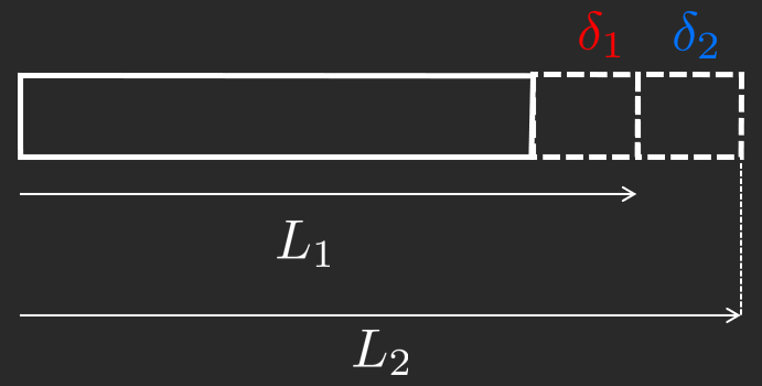
Figure 8.5.3: Two successive stretches. The second deformation \(\delta_2\) is measured against \(L_1\), not against \(L_0\).
Suppose we stretch the bar in two stages, first from \(L_0\) to \(L_1\) and then from \(L_1\) to \(L_2\), as in Figure 8.5.3. If each stage is measured against the length the bar had when that stage started, the two strains are \(\delta_1/L_0\) and \(\delta_2/L_1\), and their sum is not the total strain \((L_2 - L_0)/L_0\) measured against the original length. The reference length changed underneath us. For the small deformations of linear elasticity the discrepancy is negligible, but in metal forming, in polymer testing and anywhere else that strains reach tens of percent it is not.
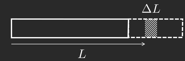
The repair is to measure every increment against the current length. A change \(\Delta L\) at the current length \(L\) contributes an increment of strain
\[
\Delta \varepsilon = \frac{\Delta L}{L}
\]
and in the limit \(\Delta L \to 0\) this becomes \(d\varepsilon = dL/L\). Integrating from the original to the final length accumulates the increments,
which is the logarithmic strain, also called true strain or Hencky strain. It adds correctly, because \(\ln(L_2/L_0) = \ln(L_2/L_1) + \ln(L_1/L_0)\) by the functional equation of the logarithm.
Figure 8.5.4: Accumulating strain increments against the current length.
The two definitions must agree when the deformation is small, and a Taylor expansion of 8.5.3 about \(\delta = 0\) shows how.
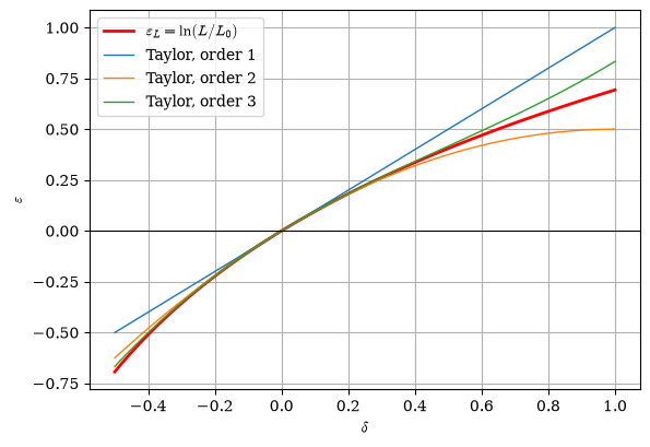
so the two measures differ only at second order. At \(\varepsilon = 0.002\), which is where steel yields, the difference is two parts in a thousand of the strain itself and no instrument in a teaching laboratory would resolve it. At \(\varepsilon = 0.5\) the difference is \(19\%\). The plot below shows where the linear approximation starts to fail.
Figure 8.5.5: Logarithmic strain against its Taylor approximations. The first-order approximation is the engineering strain.
The first-order approximation is the engineering strain itself, and it tracks the logarithmic strain closely over roughly \(\lvert\delta\rvert < 0.1\), which for \(L_0 = 1\) means strains up to about \(10\%\). The approximation is worse in compression than in tension, which is a consequence of the logarithm running to \(-\infty\) as the bar is squashed to zero length while the engineering strain merely reaches \(-1\).
Example 1: Linear and logarithmic strain compared
A rod is compressed from \(140~\text{mm}\) to \(120~\text{mm}\). Determine both strain measures.
The deformation is \(-14\%\) of the original length, well outside the range where the two measures agree, and they differ by about \(8\%\) of their own value. Which one to report depends on what the number is for: a stress analysis in the elastic range uses engineering strain because that is what the elastic constants are defined against, while a forming simulation or a tensile test taken to fracture uses logarithmic strain because only that one accumulates correctly.
Transversal strain and Poisson’s ratio
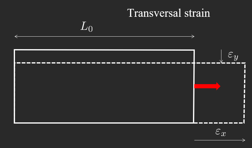
Stretching a bar makes it thinner. The contraction transverse to the load is proportional to the strain along it, and the constant of proportionality is Poisson’s ratio
with the minus sign inserted so that \(\nu\) comes out positive for ordinary materials. Measuring it requires a second instrument on the tensile specimen, either a transverse extensometer or a digital image correlation system, which is why \(\nu\) is quoted from tables far more often than it is measured.
Figure 8.5.6: Longitudinal extension accompanied by transverse contraction.
Poisson’s ratio is bounded above by \(0.5\) for an isotropic material, which is the value at which the volume stops changing. Rubber sits at \(0.4999\) and is effectively incompressible, aluminium at \(0.32\), steel between \(0.27\) and \(0.33\), and cork at almost exactly zero, which is why a cork can be pushed into a bottle neck without the sides bulging. We show in Chapter 8.9 where the limit of \(0.5\) comes from, and why \(\nu\) is the parameter that ties \(E\) and \(G\) together.
Thermal strain
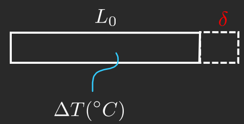
Materials deform when heated, without any load being applied. Over the temperature ranges met in ordinary engineering the deformation is proportional to the temperature change, with a proportionality constant \(\alpha\) called the coefficient of thermal expansion, measured in \(1/^\circ\text{C}\). The resulting deformation and length are
\[
\delta = L_0 \alpha \Delta T = L_0\, \varepsilon_{\text{temp}}, \qquad
L = L_0 + L_0 \alpha \Delta T
\tag{8.5.5}\]
Figure 8.5.7: Thermal expansion of an unrestrained bar.
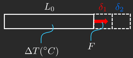
Thermal strain and mechanical strain add, since both are geometric statements about the same bar,
where the elastic part has been written using Hooke’s law, which we take up in Chapter 8.6.
Figure 8.5.8: Mechanical and thermal strain acting together.
8.5.6 is the source of a class of problems that catches students out. If a bar is free to expand, heating it produces strain but no stress, because \(\sigma = 0\) and all of \(\varepsilon_{\text{tot}}\) comes from the thermal term. If the bar is clamped at both ends so that \(\varepsilon_{\text{tot}} = 0\), heating it produces no strain but a compressive stress \(\sigma = -E\alpha\Delta T\), which for steel amounts to roughly \(2.5~\text{MPa}\) per degree. This is why bridges have expansion joints and why pipework has bends in it. It is also why a bridge rests on a roller support at one end: the roller lets the deck change length with temperature without large constraint forces, whereas a deck locked at both ends is the bar between rigid walls, and a \(30~^\circ\text{C}\) rise would put about \(75~\text{MPa}\) of compression into a steel girder.
Example 2: Shrink-fitting a hub onto a shaft
“That way it will never work itself loose, considering we have a 100 degree Celsius interference fit.”
— Alec Steele, blacksmith, restoring a power hammer
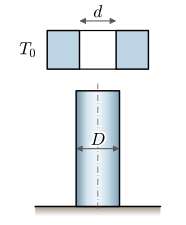
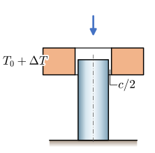
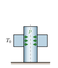
A gear, pulley or wheel can be fixed to its shaft without a key or glue by making the bore of its hub slightly smaller than the shaft. The difference in diameter is the interference\(\delta = D - d\), and once the parts are assembled the hub grips the shaft with a contact pressure that transmits torque by friction. Pushing the parts together cold needs a press and scrapes the surfaces. The alternative is to heat the hub until its bore is larger than the shaft, slide it on, and let it cool, as in Figure 8.5.9. Railways still fit steel tyres to their wheel centres the same way.
A steel hub with a bore of nominal diameter \(60~\text{mm}\) is to be shrink-fitted onto a steel shaft with the ISO fit H7/s6. The largest interference the fit allows is \(\delta = 0.072~\text{mm}\), between the smallest bore (\(60.000~\text{mm}\)) and the largest shaft (\(60.072~\text{mm}\)). We want a clearance of \(c = 0.05~\text{mm}\) during assembly, so that the hub can be slid into place before it cools onto the shaft. Determine how hot the hub must be, starting from \(T_0 = 20~^\circ\text{C}\), with \(\alpha = 12 \cdot 10^{-6}~1/^\circ\text{C}\) for steel.
(a) At room temperature the bore \(d\) is smaller than the shaft \(D\).
(b) The heated hub slides over the shaft with the clearance \(c\).
(c) Cooled, the hub grips the shaft with the pressure \(p\).
Figure 8.5.9: Shrink-fitting a hub onto a shaft, in axial section. The interference is drawn about a hundred times too large.
A free hub heated uniformly carries no stress, so by 8.5.6 every line in it stretches by the same strain \(\alpha\Delta T\), whatever its direction and wherever it lies. The circumference of the bore is such a line. Its length \(\pi d\) grows to \(\pi d(1 + \alpha\Delta T)\), so the bore diameter grows in the same proportion, exactly as if the hole were filled with steel. The hub goes on when the heated bore equals the shaft diameter plus the clearance,
\[
d\,(1 + \alpha\Delta T) = D + c
\tag{8.5.7}\]
and with \(D = d + \delta\) this is one equation for the temperature rise.
Code
d, D, c, alpha, Delta_T = sp.symbols(r'd D c alpha \Delta{T}', positive=True)delta_i = sp.symbols('delta', positive=True) # the interference D - dDelta_T_req = sp.solve(sp.Eq(d*(1+ alpha*Delta_T), D + c), Delta_T)[0]Delta_T_req = sp.simplify(Delta_T_req.subs(D, d + delta_i))ltx(r"\Delta T =", Delta_T_req)
\[ \Delta T =\dfrac{c + \delta}{\alpha d} \]
The required temperature rise is
\[
\boxed{\Delta T = \frac{\delta + c}{\alpha\, d}}
\tag{8.5.8}\]
since the bore must grow by the interference and the clearance together, and it grows by \(\alpha d\) for every degree. The hub’s outer diameter and width do not enter, since the thermal strain is the same everywhere in it. With the numbers of the problem,
\[ \begin{aligned}\Delta T &=169.4~^\circ\text{C}\\ T_{\text{hub}} = T_0 + \Delta T &=189.4~^\circ\text{C}\end{aligned} \]
The hub must be heated to about \(190~^\circ\text{C}\), which an oven or an induction heater reaches in minutes. A hub of ordinary structural steel takes this without harm. A case-hardened gear may not, because its hardness was set by tempering at a temperature of the same order, and there the clearance is kept small and the temperature checked. A blacksmith with a forge at hand tends to heat far more, and the surplus goes into clearance.
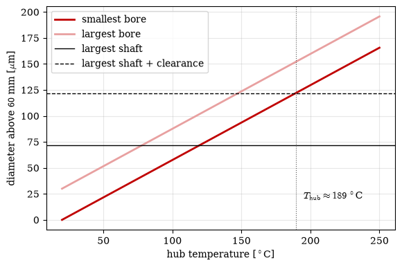
The tolerance bands of the fit make the result easy to check graphically. Figure 8.5.10 follows the bore of the hub as it heats, for the smallest and the largest bore the H7 tolerance allows, against the largest shaft the s6 tolerance allows. The hub goes on where the bore line crosses the shaft plus the clearance, and the worst case is the smallest bore on the largest shaft.
Figure 8.5.10: The bore of the heated hub against the largest shaft of an H7/s6 fit at \(60~\text{mm}\). The smallest bore reaches the shaft plus the clearance at the temperature of 8.5.8.
The red line crosses the dashed one at the computed temperature, and a hub with the largest bore gets there some forty degrees sooner. Once the hub cools, its bore tries to return to \(d\) and the shaft is in the way. Both parts then deform elastically, the hub stretched and the shaft squeezed, until they meet at a common diameter, and the contact pressure \(p\) in Figure 8.5.9 (c) is whatever it takes to hold them there. Computing it needs the stresses in a thick-walled cylinder, which we take up in the chapter on shaft–hub joints. The heating only makes assembly possible. The grip is set by the interference alone.
Alec Steele’s remark at the head of this example gives the interference in degrees. That is the temperature rise which opens the bore by exactly \(\delta\),
Stated in degrees, the claim is easy to test. Heating the whole assembly changes nothing when hub and shaft are both steel, because bore and shaft grow in the same proportion and the interference grows with them. The fit opens only if the hub runs \(100~^\circ\text{C}\) hotter than the shaft, which a hub in service seldom does unless friction or a process heats it. Within the thermal model the claim holds. It says nothing about the other ways a fit works loose, such as slip under a torque larger than the grip can carry, or fretting wear under alternating bending. Both depend on the pressure \(p\), which the shaft–hub chapter computes. Parts of different materials behave differently, as Exercise 8.5.1 shows.
Shear strain
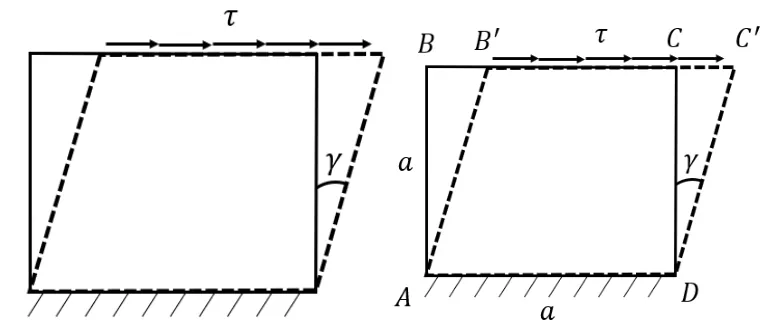
Normal strain measures the stretching of a line. Shear strain measures the change in angle between two lines that were originally perpendicular. Take the square element in Figure 8.5.11, hold its lower edge fixed and apply a shear stress along its upper edge. The square becomes a parallelogram, and the angle by which the vertical edges have tilted is the shear angle\(\gamma\).
Figure 8.5.11: A square element deformed into a parallelogram by shear.
The area is preserved by the deformation, which requires \(a^2 = a\,h\cos\gamma\) where \(h = \lvert AB'\rvert\) is the length of the deformed edge. For small angles \(\cos\gamma \approx 1\), so \(h \to a\): the edges neither stretch nor shorten, they only rotate. The upper edge has then translated by \(\delta = \lvert BB'\rvert\) over a height \(a\), and the shear strain is defined as that ratio,
which is the exact analogue of \(\varepsilon = \delta/L_0\) with the height playing the role of the reference length. Shear strain is dimensionless and, like normal strain, is small in every application this book treats.
The material relation for shear has the same form as Hooke’s law,
\[
\boxed{\tau = G\gamma}
\tag{8.5.11}\]
where \(G\) is the shear modulus. It is not an independent material property. For an isotropic material it is fixed by the Young’s modulus and the Poisson’s ratio through
\[
\boxed{G = \frac{E}{2(1+\nu)}}
\tag{8.5.12}\]
which we derive in Chapter 8.9. For steel, with \(E = 210\,000~\text{MPa}\) and \(\nu = 0.3\), this gives \(G \approx 81\,000~\text{MPa}\), so a material resists shearing roughly two and a half times less stiffly than it resists stretching. That single number explains why thin-walled sections are so much better in bending than in torsion, and it will return in Chapter 8.16 when we compare the Euler-Bernoulli and Timoshenko beam models.
Problems
Exercise 8.5.1 An aluminium hub is shrink-fitted onto a steel shaft of diameter \(40~\text{mm}\) with an interference of \(0.04~\text{mm}\). The coefficients of thermal expansion are \(\alpha_{\text{Al}} = 23 \cdot 10^{-6}~1/^\circ\text{C}\) and \(\alpha_{\text{st}} = 12 \cdot 10^{-6}~1/^\circ\text{C}\), and the workshop is at \(20~^\circ\text{C}\). Determine the hub temperature needed for a clearance of \(0.03~\text{mm}\) during assembly. In service the whole assembly warms up uniformly. At what temperature has the interference vanished, so that the hub comes loose? What changes if the materials are swapped, with a steel hub on an aluminium shaft?
Exercise 8.5.2 Instead of heating the hub, the shaft can be cooled. A steel shaft of diameter \(40~\text{mm}\) is to be fitted into a steel hub with an interference of \(0.05~\text{mm}\), and a clearance of \(0.03~\text{mm}\) is wanted during assembly. The shaft is dipped in liquid nitrogen at \(-196~^\circ\text{C}\) from room temperature \(20~^\circ\text{C}\). The coefficient of thermal expansion of steel falls with temperature, so use a mean value of \(\alpha = 9 \cdot 10^{-6}~1/^\circ\text{C}\) over this range. Is cooling the shaft enough? If it is not, how much must the hub be heated as well, with \(\alpha = 12 \cdot 10^{-6}~1/^\circ\text{C}\) above room temperature?