8.21 Fatigue
Every strength check in the preceding chapters compared a stress with a strength measured once, in a tensile test: the part was safe if the largest stress stayed below the yield strength \(R_{p0.2}\) or the tensile strength \(R_m\) of Chapter 8.6. Yet parts break in service at stresses well below both. A shaft that turns carries a bending stress that changes sign on every revolution, a car suspension arm is loaded at every bump in the road, and a pressurised cabin is loaded at every flight. A stress far too small to break the part once can break it after it has been applied a million times. This failure under repeated loading is fatigue. It is a different mechanism from creep, the slow deformation of a material held under constant load over time, most marked at high temperature: creep needs time under load, fatigue needs the load to change.
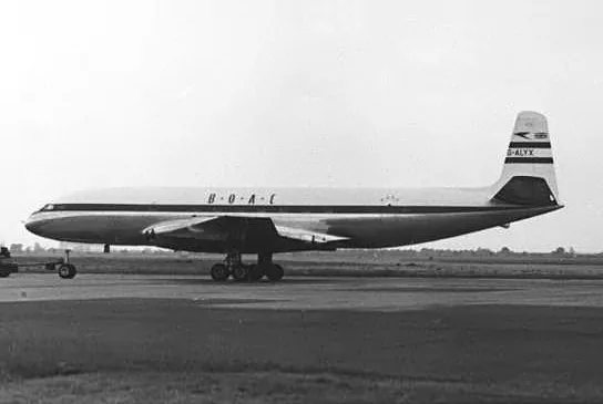
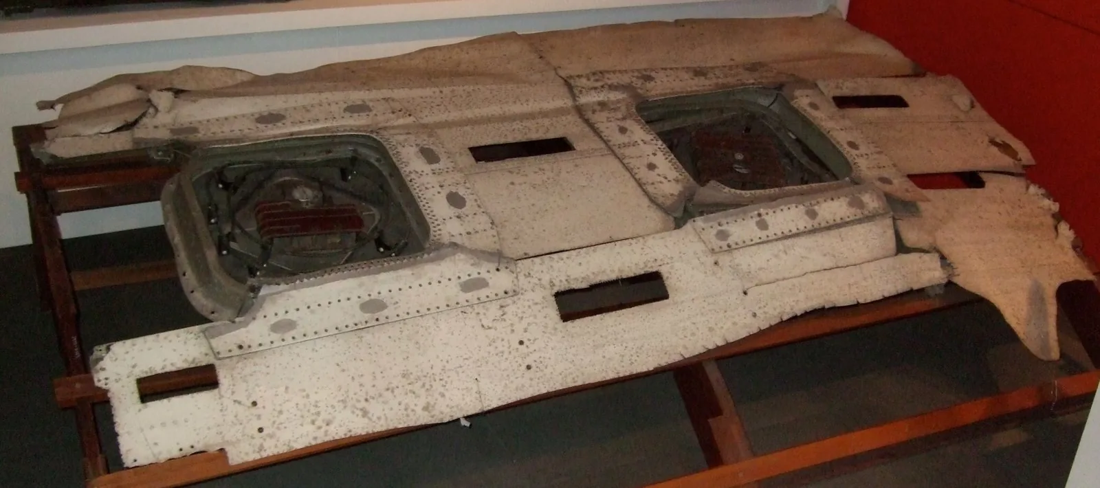
Fatigue entered engineering through the railways. In May 1842 a train returning to Paris from Versailles crashed when the axle of its leading locomotive broke, and through the following decades August Wöhler tested railway axles under repeated loads. He concluded that the range of the stress matters more than its peak and that iron and steel have a stress amplitude below which they last indefinitely [1]. The lesson has had to be relearned. In 1954 two de Havilland Comet airliners, the first jet passenger aircraft, broke up in flight from fatigue cracks driven by the pressurisation of the cabin on every flight, Figure 8.21.1, and in 1980 the semi-submersible platform Alexander L. Kielland capsized in the North Sea, killing 123 people, after a fatigue crack had grown through one of its bracings from a small fillet weld that attached a sonar fitting to it.
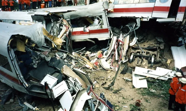
Railways met fatigue again in June 1998, when the high-speed train ICE 884 derailed at about \(200~\text{km/h}\) near Eschede in Lower Saxony, killing 101 people in the worst accident in the history of high-speed rail. Its wheels had a rubber damper between the wheel body and a thin steel tyre, the outer ring that runs on the rail, and a fatigue crack grew through one of the tyres until it broke and peeled off. The tyre lodged in the floor of the carriage and derailed it at a set of points, and the train struck the supports of a road bridge, which collapsed onto it, Figure 8.21.2. The wheels had been inspected by eye with a torch, and the crack was not found. All wheels of the type were then replaced with solid monobloc wheels. Railway workers have long checked wheels by striking them with a hammer and listening: a sound wheel rings with a clear tone, while a crack damps the vibration and the wheel sounds dull.
Fatigue does not need a new continuum model. The stresses come from the analyses of the preceding chapters, and the stress concentrations of Chapter 8.19 decide where a crack starts. What is new is how the material responds when that stress field is applied again and again. We describe a load cycle, look at how a fatigue crack starts and grows, introduce the S-N curve and the corrections that carry it from a test specimen to a real part, account for the mean stress, count the cycles of an irregular history, and work through the shaft of Chapter 8.19 once more, now as a rotating shaft.
Describing a load cycle
The simplest load history is a constant-amplitude cycle between the largest stress \(\sigma_{\max}\) and the smallest \(\sigma_{\min}\), Figure 8.21.3. Fatigue tests and design rules describe it by its mean value and its amplitude,
\[ \sigma_m = \frac{\sigma_{\max} + \sigma_{\min}}{2}, \qquad \sigma_a = \frac{\sigma_{\max} - \sigma_{\min}}{2} \tag{8.21.1}\]
or by the stress range \(\Delta\sigma = \sigma_{\max} - \sigma_{\min} = 2\sigma_a\) together with the stress ratio
\[ R = \frac{\sigma_{\min}}{\sigma_{\max}} \tag{8.21.2}\]
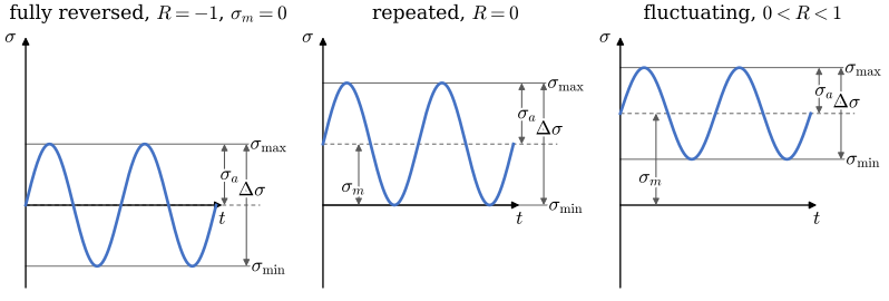
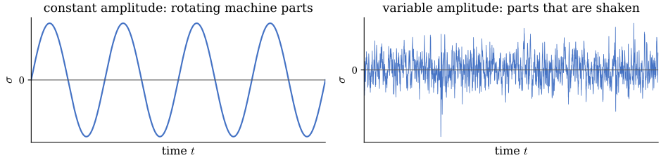
The fully reversed cycle is the one of a rotating shaft under a constant bending moment, where every point of the surface passes from tension to compression and back on every revolution. The repeated cycle is that of a gear tooth, loaded once per revolution and then unloaded. A bolt that is pretensioned and then loaded further in service follows a fluctuating cycle with a large mean stress. Swedish texts call the fully reversed cycle växlande and the repeated one pulserande. Real load histories, such as the stress in a suspension arm on a rough road, are irregular. They are reduced to a list of cycles with known amplitudes and means by counting methods, of which rainflow counting is the standard, and the methods of this chapter are then applied cycle by cycle. Figure 8.21.4 contrasts the two kinds of history.
How a fatigue crack starts and grows
A fatigue failure passes through three stages. In the first, a crack initiates. Even when the nominal stress is elastic, single grains at the surface, where they are least constrained, deform plastically by slip along favourably oriented crystal planes. Repeated slip back and forth roughens the surface into tiny intrusions and extrusions, and a microscopic crack forms. Initiation is fastest where the local stress is highest and the surface is weakest: at notches, fillets and holes, at scratches and machining marks, at inclusions in the material, at weld toes, and in a 3D-printed part at the boundaries between layers.
In the second stage the crack grows, by a small amount on every cycle, in the direction perpendicular to the largest principal stress. Each change in the loading, a stop or a period of higher load, leaves a mark on the crack face, and the crack front is preserved as a set of curved beach marks, Figure 8.21.5. The crack faces rub against each other as the load reverses, which makes this part of the fracture surface smooth and often dark. In the third stage the crack has grown so long that the remaining section can no longer carry the peak load, and it breaks suddenly in a single overload, leaving a rough, bright surface.
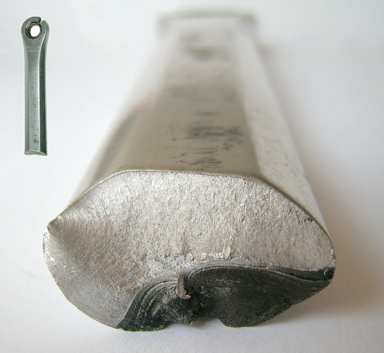
The surface of Figure 8.21.5 shows what makes fatigue dangerous. The part gave no warning by visible deformation, the final fracture looks brittle although aluminium is a ductile metal, and most of the life of the part was spent growing a crack that nobody saw.
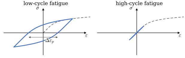
How much plastic deformation each cycle causes divides fatigue into two regimes, Figure 8.21.6. If the stress amplitude exceeds the yield strength, every cycle deforms the material plastically and traces a hysteresis loop in the stress-strain diagram, whose width is the plastic strain range \(\Delta\varepsilon_p\). Such low-cycle fatigue breaks a part within roughly \(10^3\) to \(10^4\) cycles, and it is analysed in terms of the strain, since the strain is what the loop controls; it concerns, e.g., parts heated and cooled in every start of a machine. In high-cycle fatigue the nominal stress stays elastic, the cycle runs back and forth along the straight part of the curve, and the plastic slip is confined to single grains at the surface. Most machine parts, which must last millions of cycles, are in this regime, and it is analysed in terms of the stress.
The strain-based description of low-cycle fatigue goes back to Manson and Coffin, who studied parts cracked by repeated heating and cooling [2,3]. They split the strain amplitude \(\Delta\varepsilon/2\) of the loop into its elastic and plastic parts and found that each falls as a power of the number of load reversals \(2N\), two per cycle,
\[ \frac{\Delta\varepsilon}{2} = \frac{\sigma_f'}{E}(2N)^{b} + \varepsilon_f'(2N)^{c} \tag{8.21.3}\]
The first term is the elastic strain of the S-N line of the next section, 8.21.4, divided by Young’s modulus \(E\) and written for reversals, with the fatigue strength coefficient \(\sigma_f'\) and the same exponent \(b\). The second term is the Coffin-Manson relation for the plastic strain, with the fatigue ductility coefficient \(\varepsilon_f'\), close to the true strain at fracture, and an exponent \(c\) between about \(-0.5\) and \(-0.7\). The plastic term falls much more steeply, so it dominates at short lives and the elastic term at long ones. The two are equal at the transition life, which is longer for a soft, ductile steel than for a hard one. The rest of the chapter treats high-cycle fatigue, where only the elastic term is left.
The S-N curve
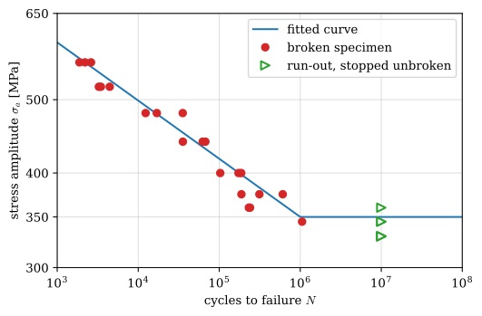
The fatigue strength of a material is measured by loading specimens with constant-amplitude cycles until they break. The classical test, due to Wöhler, bends a polished cylindrical specimen while it rotates, so that every point of its surface sees a fully reversed cycle once per revolution, and counts the revolutions to failure. Repeating the test at several amplitudes gives the S-N curve, also called the Wöhler curve: the stress amplitude \(\sigma_a\) against the number of cycles to failure \(N\), on logarithmic axes. Figure 8.21.7 shows the test.
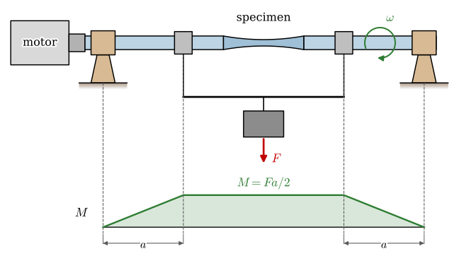
The shaft between the load bearings is in four-point bending, with no shear force and the same moment along the whole specimen, so the specimen breaks where it is thinnest. At its smallest diameter \(d\) the surface carries the bending stress of 8.16.11,
\[ \sigma_a = \frac{32M}{\pi d^3} = \frac{16Fa}{\pi d^3} \]
and as the shaft turns, every point of the surface passes from the tension side to the compression side and back once per revolution, so this stress is the amplitude of a fully reversed cycle. Each specimen gives one point of the curve, the amplitude it was tested at and the number of revolutions it survived, Figure 8.21.9. A specimen that has not broken after a set number of cycles, often \(10^7\), is stopped and recorded as a run-out.
Code
rng = np.random.default_rng(7)
R_m_d, f_d, se_d = 700, 0.85, 350                    # a polished steel specimen, @eq-endurance-estimate
a_d = (f_d*R_m_d)**2/se_d
b_d = -np.log10(f_d*R_m_d/se_d)/3
N_runout = 1e7

levels = np.repeat([560, 520, 480, 440, 400, 375, 360, 345, 330], 3)
N_med = (levels/a_d)**(1/b_d)                         # the median life on the sloping line
N_test = N_med*10**(0.25*rng.standard_normal(levels.size))    # the scatter of real tests
se_own = se_d*(1 + 0.04*rng.standard_normal(levels.size))     # each specimen's own limit
broke = (levels > se_own) & (N_test < N_runout)

N_line = np.logspace(3, 8, 300)
fig, ax = plt.subplots(figsize=(6, 3.8))
ax.loglog(N_line, np.where(N_line < 1e6, a_d*N_line**b_d, se_d), color='C0', lw=1.5,
          label='fitted curve')
ax.loglog(N_test[broke], levels[broke], 'o', color='C3', ms=6, label='broken specimen')
ax.loglog(np.full((~broke).sum(), N_runout), levels[~broke], '>', color='C2', ms=7,
          mfc='white', mew=1.5, label='run-out, stopped unbroken')
ax.set_xlabel('cycles to failure $N$')
ax.set_ylabel(r'stress amplitude $\sigma_a$ [MPa]')
ax.set_xlim(1e3, 1e8)
ax.set_ylim(300, 650)
ax.set_yticks([300, 350, 400, 500, 650], ['300', '350', '400', '500', '650'])
ax.minorticks_off()
ax.grid(True, which='both', alpha=0.4)
ax.legend(loc='upper right')
plt.show()Data of this kind is expensive. A rotating-bending machine runs at around 50 revolutions per second, so a single specimen taken to \(10^7\) cycles occupies it for more than two days, and one taken to \(10^8\) cycles for more than three weeks. The scatter means that every amplitude needs several specimens, so one S-N curve with its knee takes a few dozen specimens, all machined and polished alike, and months of machine time. The curve then holds only for that material, that surface, that size and a zero mean stress. Yet there is no way around it: every fatigue calculation in this chapter starts from a measured curve, and even the estimate below is a fit to such tests. This is why fatigue data is collected in handbooks and guarded by the companies that paid for it.
A fatigue test at Jönköping University
The rotating-bending machine is the classical test, but most fatigue tests today run in a servohydraulic machine such as the one in Figure 8.21.10 (a), in the materials and manufacturing department of the School of Engineering at Jönköping University. Two columns carry a crosshead, from which the upper grip hangs below a load cell that measures the force. The lower grip sits on a hydraulic actuator in the base, which pushes and pulls the specimen. Oil at high pressure comes through the blue hoses from the hydraulic power unit on the right, and it also clamps the specimen in the two hydraulic wedge grips of Figure 8.21.10 (b). A controller compares the measured force with the commanded one and adjusts a servo valve on the actuator continuously, so the machine follows any prescribed force history: a sine for a constant-amplitude test, or a recorded history from a vehicle for a variable-amplitude one, Figure 8.21.4.
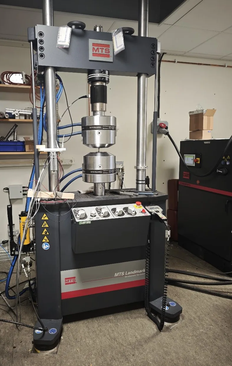
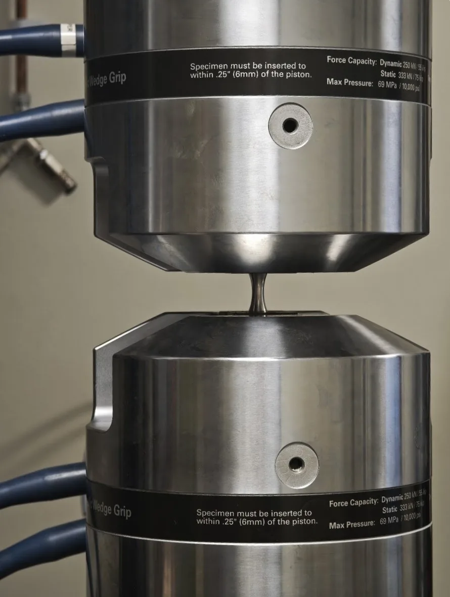
The specimen is loaded axially, in tension and compression, and the whole of its waist carries the same stress. In rotating bending only a thin layer at the surface is highly stressed, so an axial test finds a defect to start a crack from more easily. This is why the load factor of the previous section is \(k_c = 0.85\) for an axial load.
The machine stands in a former cleaning closet. Its reinforced concrete floor is the roof of a bomb shelter built during the Cold War, and that floor, able to take the weight of the machine and the forces it shakes into the ground, is why the room was chosen.
When the photographs were taken, the controller was cycling the force between \(+20.7\) and \(-21.3~\text{kN}\), a fully reversed cycle with \(R \approx -1\), and it had counted \(N = 1\,859\,164\) cycles after the running time \(t = 25~\text{h}\;49~\text{min}\;27~\text{s}\). A sinusoidal force of amplitude \(F_a\) and frequency \(f\), and the number of cycles it has applied, are
\[ F(t) = F_a \sin(2\pi f t), \qquad N = f t \]
so the record gives the test frequency \(f = N/t\), and the time a run-out at \(10^7\) cycles takes is \(t_{10^7} = 10^7/f\).
Code
N_count = 1859164
t_run = 25*3600 + 49*60 + 27                 # s
f_test = N_count/t_run
t_runout = 1e7/f_test/(24*3600)              # days

ltx(r"f = \frac{N}{t} =", f_test, r"~\text{Hz}, \qquad t_{10^7} = \frac{10^7}{f} =", t_runout,
    r"~\text{days}", precision=3)
\[ f = \frac{N}{t} =20.0~\text{Hz}, \qquad t_{10^7} = \frac{10^7}{f} =5.79~\text{days} \]
The machine runs at \(20~\text{Hz}\), and the specimen, a day into its test, has covered less than a fifth of the way to a run-out, which would take almost six days. Figure 8.21.11 redraws two of the records the controller displays, the force over a few cycles and the force against the displacement of the actuator. The displacement follows the force through the stiffness \(k\) of the specimen and the grips, \(\delta = F/k\), and the measured peaks, \(\pm 21~\text{kN}\) at about \(\pm 0.13~\text{mm}\), give \(k \approx 160~\text{kN/mm}\).
Code
F_a, k_train = 21.0, 21.0/0.13             # kN, kN/mm, from the controller's peak readings
t = np.linspace(0, 0.2, 400)                  # s, four cycles at 20 Hz
F = F_a*np.sin(2*np.pi*f_test*t)

fig, (ax1, ax2) = plt.subplots(1, 2, figsize=(9, 3.4))
ax1.plot(1e3*t, F, color='C0', lw=2)
ax1.axhline(0, color='0.35', lw=0.8)
ax1.set_xlabel('time $t$ [ms]')
ax1.set_ylabel('axial force $F$ [kN]')
ax1.set_xticks([0, 50, 100, 150, 200])
ax1.set_yticks([-21, -10, 0, 10, 21])
ax1.set_xlim(0, 200)
ax1.grid(True, alpha=0.4)
ax2.plot(F/k_train, F, color='C3', lw=2)
ax2.axhline(0, color='0.35', lw=0.8)
ax2.axvline(0, color='0.35', lw=0.8)
ax2.set_xlabel(r'axial displacement $\delta$ [mm]')
ax2.set_ylabel('axial force $F$ [kN]')
ax2.set_xticks([-0.13, -0.05, 0, 0.05, 0.13])
ax2.set_yticks([-21, -10, 0, 10, 21])
ax2.set_xlim(-0.16, 0.16)
ax2.grid(True, alpha=0.4)
fig.tight_layout()
plt.show()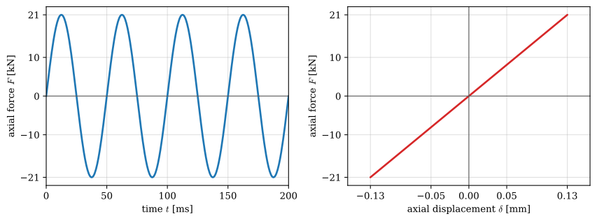
The force-displacement record has no loop. Every cycle runs up and down the same straight line, the elastic line of Figure 8.21.6, so the specimen is in high-cycle fatigue: no plastic strain can be measured, and the damage builds up in single grains at the surface until a crack starts. The record will look the same until shortly before the specimen breaks, when the growing crack lowers its stiffness and the line starts to tilt.
Figure 8.21.12 shows the whole curve of a steel, from a single cycle, where the amplitude that breaks the specimen equals the tensile strength \(R_m\), to \(10^8\) cycles. Below about \(10^3\) cycles lies the low-cycle fatigue of the previous section. Between \(10^3\) and \(10^6\) cycles the part has a finite life that the curve predicts, and beyond the knee its life is infinite as long as the amplitude stays below the endurance limit.
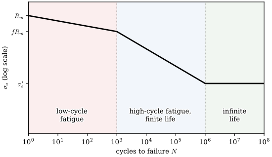
Between about \(10^3\) and \(10^6\) cycles the S-N curve of a steel is close to a straight line on the double logarithmic axes, as Basquin observed in 1910 [4],
\[ \sigma_a = a N^b \tag{8.21.4}\]
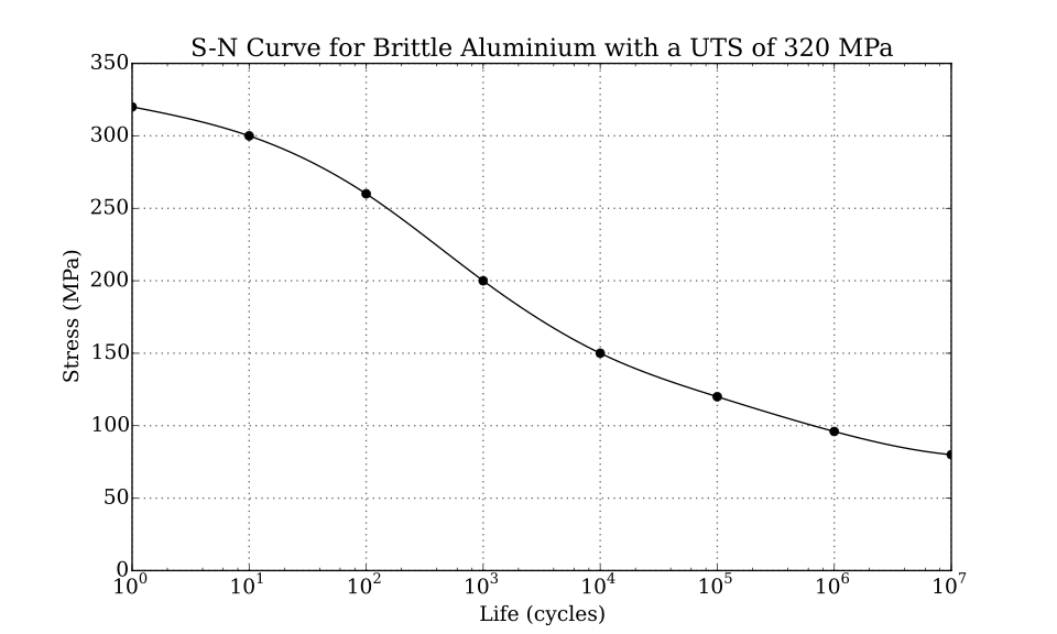
with a negative exponent \(b\), typically between \(-0.05\) and \(-0.15\). Near \(10^6\) to \(10^7\) cycles the curve of most steels bends over into a horizontal line, and below this endurance limit \(\sigma_e'\) a polished specimen lasts indefinitely. Aluminium alloys, most other non-ferrous metals and polymers show no such knee: their curve keeps falling, and their fatigue strength is quoted at a stated number of cycles, often \(5 \cdot 10^8\), Figure 8.21.13.
When no test data is available, Shigley gives an estimate for steels from the tensile strength alone [5]. The endurance limit of the polished specimen is about half the tensile strength,
\[ \sigma_e' \approx \begin{cases} 0.5\,R_m & R_m \le 1400~\text{MPa} \\ 700~\text{MPa} & R_m > 1400~\text{MPa} \end{cases} \tag{8.21.5}\]
and the line 8.21.4 is drawn from the strength \(f R_m\) at \(N = 10^3\) cycles to the endurance limit \(\sigma_e\) at \(N = 10^6\), where \(f\) falls from about \(0.9\) for \(R_m = 500~\text{MPa}\) to \(0.8\) for very strong steels. The two points fix the constants,
\[ a = \frac{(f R_m)^2}{\sigma_e}, \qquad b = -\frac{1}{3}\log_{10}\frac{f R_m}{\sigma_e} \tag{8.21.6}\]
and solving 8.21.4 for \(N\) gives the life at a given amplitude above the endurance limit,
\[ N = \left(\frac{\sigma_a}{a}\right)^{1/b} \tag{8.21.7}\]
Figure 8.21.14 draws the estimate for a steel with \(R_m = 700~\text{MPa}\), for which \(f \approx 0.85\), together with the curve of the shaft of Example 1 below, whose endurance limit has been reduced by the corrections of the next section.
Code
def sn_curve(N, R_m, sigma_e, f):
    """The stress amplitude at the life N: @eq-basquin above 10^6 cycles, sigma_e beyond."""
    a = (f*R_m)**2/sigma_e
    b = -np.log10(f*R_m/sigma_e)/3
    return np.where(N < 1e6, a*N**b, sigma_e)

R_m, f_sn = 700, 0.85
N = np.logspace(3, 8, 300)

fig, ax = plt.subplots(figsize=(6, 3.8))
ax.loglog(N, sn_curve(N, R_m, 0.5*R_m, f_sn), color='C0', lw=2,
          label=r"polished specimen, $\sigma_e' = 0.5\,R_m$")
ax.loglog(N, sn_curve(N, R_m, 238, f_sn), color='C1', lw=2,
          label=r'machined shaft, $\sigma_e = 238$ MPa')
ax.axvline(1e6, color='0.35', lw=0.8, ls=':')
ax.set_xlabel('cycles to failure $N$')
ax.set_ylabel(r'stress amplitude $\sigma_a$ [MPa]')
ax.set_xlim(1e3, 1e8)
ax.set_ylim(150, 700)
ax.set_yticks([150, 238, 350, 595, 700], ['150', '238', '350', '595', '700'])
ax.minorticks_off()
ax.grid(True, which='both', alpha=0.4)
ax.legend()
plt.show()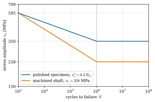
Scatter and the design curve
The curves give the median life, which half of all parts fail to reach. Behind them lies the scatter of Figure 8.21.9, where the lives at one amplitude spread over a factor of ten. The logarithm of the life at a given amplitude is close to normally distributed, so the scatter is measured by the standard deviation \(s\) of \(\log_{10} N\). Design codes fit the finite-life data with 8.21.4 solved for the life, a straight line in the logarithms,
\[ \log_{10} N = A - m\log_{10}\sigma_a, \qquad m = -\frac{1}{b} \]
and treat \(N\) as the scattered quantity, since the machine sets the amplitude and the test measures the life. The \(n_s\) broken specimens leave the residuals \(r_j = \log_{10} N_j - (A - m\log_{10}\sigma_{a,j})\) about the fitted line, and their standard deviation is
\[ s = \sqrt{\frac{1}{n_s - 2}\sum_{j=1}^{n_s} r_j^2} \]
where the two fitted constants \(A\) and \(m\) use up two of the \(n_s\) degrees of freedom. The design curve runs \(k\) standard deviations below the mean,
\[ \log_{10} N_d = A - ks - m\log_{10}\sigma_a \tag{8.21.8}\]
and a part fails before \(N_d\) with the probability \(\Phi(-k)\) of the standard normal distribution, \(2.3~\%\) for \(k = 2\) and \(1~\%\) for \(k = 2.33\). At a given amplitude the design curve shortens the life by the factor \(N_d/N = 10^{-ks}\). At a given life it lowers the amplitude by the factor \(10^{-ks/m}\), which follows from setting the two logarithms of the life equal. We fit the specimens of Figure 8.21.9 that broke on the sloping line, at \(400~\text{MPa}\) and above, and evaluate both factors for \(k = 2\).
Code
fit = broke & (levels >= 400)                    # broken on the sloping line
x, y = np.log10(levels[fit]), np.log10(N_test[fit])
slope, A_fit = np.polyfit(x, y, 1)                # the least-squares line of log N on log sigma_a
m_fit = -slope
s_fit = np.sqrt(np.sum((y - (A_fit - m_fit*x))**2)/(x.size - 2))
k_dc = 2

ltx(r"n_s =", int(fit.sum()), r", \quad m =", m_fit, r", \quad s =", s_fit,
    r", \quad 10^{-ks} =", 10**(-k_dc*s_fit), r", \quad 10^{-ks/m} =", 10**(-k_dc*s_fit/m_fit),
    precision=3)
\[ n_s =15, \quad m =13.2, \quad s =0.163, \quad 10^{-ks} =0.472, \quad 10^{-ks/m} =0.945 \]
Code
sig = np.linspace(395, 600, 100)
fig, ax = plt.subplots(figsize=(6, 3.8))
ax.loglog(10**(A_fit - m_fit*np.log10(sig)), sig, color='C0', lw=2, label='mean curve, 50 % fail')
ax.loglog(10**(A_fit - k_dc*s_fit - m_fit*np.log10(sig)), sig, color='C3', lw=2, ls='--',
          label=r'design curve, $k = 2$, 2.3 % fail')
ax.loglog(N_test[fit], levels[fit], 'o', color='0.3', ms=5, label='broken specimens')
ax.set_xlabel('cycles to failure $N$')
ax.set_ylabel(r'stress amplitude $\sigma_a$ [MPa]')
ax.set_xlim(1e3, 1e6)
ax.set_ylim(380, 620)
ax.set_yticks([400, 480, 560, 620], ['400', '480', '560', '620'])
ax.minorticks_off()
ax.grid(True, which='both', alpha=0.4)
ax.legend(loc='upper right')
fig.tight_layout()
plt.show()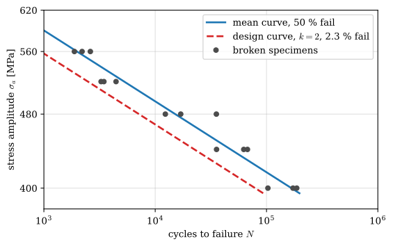
The fit returns the slope \(m = 13.2\), close to the \(13.0\) of the curve the lives were simulated from, and \(s = 0.16\). Two standard deviations below the median roughly halve the life but lower the amplitude by only \(6~\%\), because the curve is flat: a small step down in stress is a long step along in life. The reliability factor \(k_e\) of the next section acts on the stress for this reason, and a value close to one already buys a large margin of life. The simulation drew the lives with \(s = 0.25\), and fifteen specimens estimated it as \(0.16\). With few specimens the standard deviation is itself uncertain, and some codes therefore state a confidence along with the probability of survival.
Design codes for welded steel structures publish their curves in this form. DNV-RP-C203 for offshore structures and BS 7608 place them two standard deviations below the mean of the test data, a survival probability of \(97.7~\%\) [6,7]. Eurocode 3 names each welded detail by its detail category, the stress range at \(2 \cdot 10^6\) cycles that \(95~\%\) of such details survive, estimated with \(75~\%\) confidence [8]. These curves are written for the stress range \(\Delta\sigma\) and fall with the slope \(m = 3\), far steeper than that of a polished specimen, because a weld toe already holds a crack-like defect and almost the whole life is spent growing it, as the end of this chapter shows. They apply at any mean stress, since the residual stresses at a weld reach the yield strength whatever the load does. For a welded part the designer reads the life off such a curve and has no need to test.
From the test specimen to the part
A real part differs from the polished specimen of the rotating-bending test in its surface, its size and the way it is loaded. Marin collected these differences into correction factors that multiply the endurance limit of the specimen [5],
\[ \sigma_e = k_a k_b k_c k_d k_e k_f\,\sigma_e' \tag{8.21.9}\]
The surface factor \(k_a\) accounts for the roughness of the surface, where cracks start. It is fitted as \(k_a = a_s R_m^{b_s}\) with \(R_m\) in MPa and the constants of Table 8.21.1. A rough surface harms a strong steel most, since a strong steel is more sensitive to small notches, and Figure 8.21.16 shows that a forged surface can throw away almost the whole advantage of a high tensile strength.
| Surface finish | \(a_s\) | \(b_s\) |
|---|---|---|
| Ground | \(1.58\) | \(-0.085\) |
| Machined or cold-drawn | \(4.51\) | \(-0.265\) |
| Hot-rolled | \(57.7\) | \(-0.718\) |
| As-forged | \(272\) | \(-0.995\) |
Code
R = np.linspace(300, 1400, 200)
finishes = [('ground', 1.58, -0.085), ('machined or cold-drawn', 4.51, -0.265),
            ('hot-rolled', 57.7, -0.718), ('as-forged', 272, -0.995)]

fig, ax = plt.subplots(figsize=(6, 3.6))
for (name, a_s, b_s), c in zip(finishes, ('C0', 'C1', 'C2', 'C3')):
    ax.plot(R, np.minimum(a_s*R**b_s, 1), color=c, lw=2, label=name)
ax.set_xlabel(r'tensile strength $R_m$ [MPa]')
ax.set_ylabel(r'surface factor $k_a$')
ax.set_xticks([300, 600, 900, 1200, 1400])
ax.set_yticks([0, 0.25, 0.5, 0.75, 1])
ax.set_xlim(300, 1400)
ax.set_ylim(0, 1.05)
ax.grid(True, alpha=0.4)
ax.legend()
plt.show()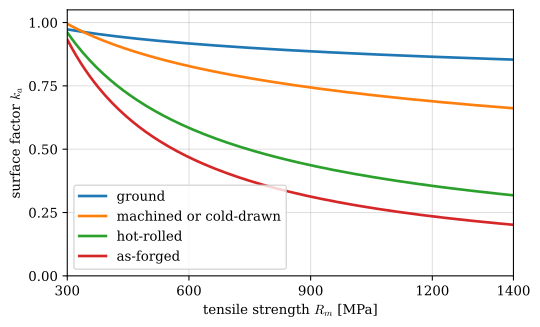
The size factor \(k_b\) accounts for the larger volume of highly stressed material in a thick part, which is more likely to contain a defect from which a crack can start. For round parts in bending or torsion
\[ k_b = 1.24\,d^{-0.107}, \qquad 2.79 \le d \le 51~\text{mm} \]
with \(d\) in millimetres, and \(k_b = 1\) for an axial load, which stresses the whole section equally. The load factor \(k_c\) converts the endurance limit measured in bending to other loads: \(k_c = 1\) in bending, \(0.85\) for an axial load and \(0.59\) for torsion. The temperature factor \(k_d\) falls below one at high temperatures. The reliability factor \(k_e\) moves the median curve down to a stated probability of survival, \(k_e = 1\) for \(50~\%\), \(0.897\) for \(90~\%\) and \(0.814\) for \(99~\%\). The miscellaneous-effects factor \(k_f\) collects everything else, e.g., corrosion, residual stresses and plating, and is one unless data says otherwise. It is unrelated to the fatigue notch factor \(K_f\) below, despite the similar symbol.
A notch is not part of 8.21.9. Its effect is applied to the stress, by multiplying the nominal stress amplitude with the fatigue notch factor \(K_f = 1 + q(K_t - 1)\) of 8.19.8, which accounts for the notch sensitivity \(q\) of the material.
The safety factor in Björk’s handbook
Swedish practice, as collected in Björk’s handbook [9], writes the same corrections as a single factor of safety against the fatigue limit,
\[ s = \frac{\lambda\delta\chi\,\sigma_D}{\varphi\left[1 + q(K_t - 1)\right]\sigma_{\text{nom}}} \tag{8.21.10}\]
The numerator is the fatigue limit of the part. The fatigue limit \(\sigma_D\) of the material for the type of loading is read from the material tables of the handbook and reduced by three factors: the surface factor \(\chi\), which plays the role of \(k_a\); the geometric size factor \(\delta\), which accounts for the stress gradient in a thick part like \(k_b\); and the technological size factor \(\lambda\), which accounts for the lower strength of the material in a thick blank, where heat treatment and forming reach the core less effectively. The denominator is the largest stress the part sees: the nominal stress \(\sigma_{\text{nom}}\) from the elementary formulas of the preceding chapters, multiplied by the fatigue notch factor \(K_f = 1 + q(K_t - 1)\) of 8.19.8 and by the shock factor \(\varphi \ge 1\), which raises the load for machines that run with impacts. Apart from the shock factor, 8.21.10 is the fully reversed case of 8.21.11 in Swedish notation, and the handbook tabulates the values of every factor.
The mean stress and the Haigh diagram
The S-N curve is measured with fully reversed cycles, \(\sigma_m = 0\). A tensile mean stress holds a crack open and lets it grow faster, so it lowers the amplitude a part can endure, while a compressive mean stress closes the crack and helps. Tested at the same amplitude and different mean stresses, the specimens give the family of S-N curves of Figure 8.21.17.
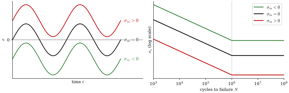
The combinations of \(\sigma_a\) and \(\sigma_m\) that a part endures indefinitely are drawn in the Haigh diagram, with the mean stress on the horizontal axis and the amplitude on the vertical, Figure 8.21.20 in Example 1 below. A failure line runs from the endurance limit \(\sigma_e\) on the amplitude axis, where the load is fully reversed, to a static strength on the mean axis, where there is no amplitude left at all.
The straight line to the tensile strength is the Goodman line [10]. With a factor of safety \(n\) applied to both stresses, a load cycle is safe if
\[ \frac{\sigma_a}{\sigma_e} + \frac{\sigma_m}{R_m} = \frac{1}{n} \tag{8.21.11}\]
defines an \(n\) above the required value. Test data fall mostly between the Goodman line and the Gerber parabola, \(n\sigma_a/\sigma_e + (n\sigma_m/R_m)^2 = 1\), so Goodman is the somewhat conservative choice and the common one in design. The Soderberg line replaces \(R_m\) by the yield strength and is more conservative still. A part must also not yield on its first cycle, which requires \(\sigma_a + \sigma_m < R_{p0.2}\), the Langer line from \(R_{p0.2}\) on one axis to \(R_{p0.2}\) on the other.
8.21.11 also converts a cycle with a mean stress into a fully reversed cycle that is equally damaging, with the amplitude
\[ \sigma_{ar} = \frac{\sigma_a}{1 - \sigma_m/R_m} \tag{8.21.12}\]
which can be entered into the S-N curve to estimate a finite life.
When the stress at the critical point is multiaxial, as at the surface of a shaft in bending and torsion, Shigley combines the components into two von Mises stresses, one from the amplitudes and one from the means,
\[ \sigma_a' = \sqrt{\left(K_f\sigma_a\right)^2 + 3\left(K_{fs}\tau_a\right)^2}, \qquad \sigma_m' = \sqrt{\left(K_f\sigma_m\right)^2 + 3\left(K_{fs}\tau_m\right)^2} \tag{8.21.13}\]
and uses them in 8.21.11 in place of \(\sigma_a\) and \(\sigma_m\) [5]. Since the combination already accounts for the type of load, the load factor is then \(k_c = 1\).
Varying amplitude and the Palmgren-Miner rule
Most parts see cycles of many amplitudes. The simplest way to combine them is the linear damage rule proposed by Palmgren for ball bearings in 1924 and by Miner for aircraft structures in 1945 [11,12]. A cycle at an amplitude whose life is \(N_i\) consumes the fraction \(1/N_i\) of the life, so \(n_i\) such cycles consume \(n_i/N_i\), and the part fails when the fractions add up to one,
\[ D = \sum_i \frac{n_i}{N_i} = 1 \tag{8.21.14}\]
The rule ignores the order of the cycles, although a few large cycles early in life start a crack that the later small cycles then grow, and it counts cycles below the endurance limit as harmless, which they are not once a crack exists. Measured damage sums at failure scatter widely around one, and design codes often set the limit lower, or continue the S-N line below the knee for variable-amplitude loading. Taken with these reservations, 8.21.14 is the standard tool for an estimate.
Counting the cycles of an irregular history
8.21.14 needs a list of cycles with their amplitudes and means, and an irregular history such as the one of Figure 8.21.4 does not provide one directly. Rainflow counting, introduced by Matsuishi and Endo [13] and standardised in ASTM E1049 [14], pairs the peaks and valleys of the history so that every closed loop of the stress-strain path of Figure 8.21.6 is counted once, as a cycle with its own range and mean. Only the extremes of the stress matter, so the history is first reduced to its turning points, the alternating peaks and valleys \(S_1, S_2, \ldots\).
The four-point form of the method reads the turning points in order and examines the last four, \(S_1\) to \(S_4\), after each new one. The inner pair \(S_2, S_3\) forms a closed cycle if its range is no larger than that of either neighbour,
\[ |S_3 - S_2| \le |S_2 - S_1| \qquad\text{and}\qquad |S_3 - S_2| \le |S_4 - S_3| \]
since the stress then runs from \(S_2\) to \(S_3\) and returns past \(S_2\) on its way to \(S_4\), closing a small loop inside the larger excursion from \(S_1\) to \(S_4\). The pair is recorded as one cycle with the extremes \(S_2\) and \(S_3\) and removed, so that \(S_1\) joins \(S_4\) directly, and the test is repeated on the new last four. Turning points that never close a cycle remain as a residue, and each step between neighbouring residue points counts as half a cycle. A block that is measured once and applied again and again is started and ended at its largest peak. Its residue then runs from that peak down to the lowest valley and back, the two halves of the largest cycle, and nothing is left unpaired.
def rainflow(S):
    """Rainflow cycles of the turning points S, as (index, index, count) triples.

    The stack holds the turning points that are not yet paired. Whenever the inner
    range of its last four is no larger than both outer ranges, the inner pair has
    closed a loop: it is a full cycle and leaves the stack. The residue left at the
    end counts as half cycles between neighbours.
    """
    stack, cycles = [], []
    for i in range(len(S)):
        stack.append(i)
        while len(stack) >= 4:
            i1, i2, i3, i4 = stack[-4:]
            inner = abs(S[i3] - S[i2])
            if inner <= abs(S[i2] - S[i1]) and inner <= abs(S[i4] - S[i3]):
                cycles.append((i2, i3, 1.0))
                del stack[-3:-1]
            else:
                break
    cycles += [(i, j, 0.5) for i, j in zip(stack[:-1], stack[1:])]
    return cycles, stack
Figure 8.21.18 applies it to a block of nine turning points that starts and ends at its largest peak, \(340~\text{MPa}\).
Code
S_block = np.array([340, -100, 180, 20, 260, -240, 120, -40, 340])     # MPa
cycles, residue = rainflow(S_block)
pairs = [(i, j) for i, j, n in cycles if n == 1.0] + [(residue[0], residue[1])]

fig, ax = plt.subplots(figsize=(7, 3.6))
turn = np.arange(S_block.size)
ax.plot(turn, S_block, color='0.55', lw=1.2, zorder=1)
for c, (num, (i, j)) in zip(('C0', 'C1', 'C2', 'C3'), enumerate(pairs, 1)):
    shown = [i, j] if num < len(pairs) else residue
    lo, hi = sorted(S_block[[i, j]])
    ax.plot(shown, S_block[shown], 'o', color=c, ms=9, zorder=3, label=f'cycle {num}: {lo} to {hi} MPa')
    if num < len(pairs):                       # the loop closes where the history next passes S_i
        for p in range(j, S_block.size - 1):
            s_lo, s_hi = sorted(S_block[p:p+2])
            if s_lo <= S_block[i] <= s_hi:
                x_close = p + (S_block[i] - S_block[p])/(S_block[p+1] - S_block[p])
                break
        ax.plot([i, x_close], [S_block[i]]*2, color=c, lw=1.5, ls=':', zorder=2)
ax.axhline(0, color='0.35', lw=0.8)
ax.set_xticks(turn)
ax.set_xlim(-0.3, 8.3)
ax.set_xlabel('turning point')
ax.set_ylabel(r'stress $\sigma$ [MPa]')
ax.set_yticks([-240, -100, 0, 180, 340])
ax.grid(True, alpha=0.4)
ax.legend(loc='center left', bbox_to_anchor=(1.01, 0.5), fontsize=9)
fig.tight_layout()
plt.show()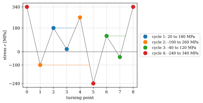
The block holds four cycles: two small excursions, cycles 1 and 3, and the larger cycle 2 lie inside the outer cycle 4, which spans the whole block. Let the block be the stress at the critical point of a steel part with \(R_m = 700~\text{MPa}\), whose endurance limit after the corrections of 8.21.9 is \(\sigma_e = 200~\text{MPa}\) and whose S-N line has \(f = 0.85\). A cycle \(i\) with the extremes \(S_{\min,i}\) and \(S_{\max,i}\) has the amplitude and mean of 8.21.1, and 8.21.12 turns it into an equally damaging fully reversed amplitude,
\[ \sigma_{a,i} = \frac{S_{\max,i} - S_{\min,i}}{2}, \qquad \sigma_{m,i} = \frac{S_{\max,i} + S_{\min,i}}{2}, \qquad \sigma_{ar,i} = \frac{\sigma_{a,i}}{1 - \sigma_{m,i}/R_m} \]
A cycle above the endurance limit has the life \(N_i = (\sigma_{ar,i}/a)^{1/b}\) of 8.21.7, with \(a\) and \(b\) from 8.21.6, and a cycle below it is taken as harmless, \(N_i = \infty\). One block adds the damage \(D_b = \sum_i n_i/N_i\) of 8.21.14, and the part lasts \(1/D_b\) blocks.
Code
from IPython.display import Markdown

R_mb, sigma_eb, f_b = 700, 200, 0.85
a_b = (f_b*R_mb)**2/sigma_eb                                     # @eq-basquin-constants
b_b = -np.log10(f_b*R_mb/sigma_eb)/3

def sci(x):
    """A number as LaTeX in powers of ten, 9.04e+05 -> 9.04 \\cdot 10^{5}."""
    mantissa, exponent = f"{x:.2e}".split("e")
    return f"{float(mantissa):.3g} \\cdot 10^{{{int(exponent)}}}"

rows, D_b = [], 0
for num, (i, j) in enumerate(pairs, 1):
    S_min, S_max = sorted(S_block[[i, j]])
    s_a, s_m = (S_max - S_min)/2, (S_max + S_min)/2
    s_ar = s_a/(1 - s_m/R_mb)                                     # @eq-equivalent-amplitude
    N_i = (s_ar/a_b)**(1/b_b) if s_ar > sigma_eb else np.inf     # @eq-life, harmless below sigma_e
    D_b += 1/N_i                                                  # @eq-miner, one of each cycle per block
    rows.append(f"| {num} | {S_min} | {S_max} | {s_a:.0f} | {s_m:.0f} | {s_ar:.0f} | "
                + (f"${sci(N_i)}$ | ${sci(1/N_i)}$ |" if np.isfinite(N_i) else "$\\infty$ | $0$ |"))

Markdown("| cycle | $S_{\\min}$ [MPa] | $S_{\\max}$ [MPa] | $\\sigma_a$ [MPa] | $\\sigma_m$ [MPa] "
"| $\\sigma_{ar}$ [MPa] | $N_i$ | $n_i/N_i$ |\n|---|---|---|---|---|---|---|---|\n" + "\n".join(rows))| cycle | \(S_{\min}\) [MPa] | \(S_{\max}\) [MPa] | \(\sigma_a\) [MPa] | \(\sigma_m\) [MPa] | \(\sigma_{ar}\) [MPa] | \(N_i\) | \(n_i/N_i\) |
|---|---|---|---|---|---|---|---|
| 1 | 20 | 180 | 80 | 100 | 93 | \(\infty\) | \(0\) |
| 2 | -100 | 260 | 180 | 80 | 203 | \(9.04 \cdot 10^{5}\) | \(1.11 \cdot 10^{-6}\) |
| 3 | -40 | 120 | 80 | 40 | 85 | \(\infty\) | \(0\) |
| 4 | -240 | 340 | 290 | 50 | 312 | \(5.94 \cdot 10^{4}\) | \(1.68 \cdot 10^{-5}\) |
Code
ltx(r"a =", a_b, r"~\text{MPa}, \quad b =", b_b, r", \quad D_b =", D_b,
    r", \quad \frac{1}{D_b} =", 1/D_b, r"~\text{blocks}", precision=3)
\[ a =1.77 \cdot 10^{3}~\text{MPa}, \quad b =-0.158, \quad D_b =1.79 \cdot 10^{-5}, \quad \frac{1}{D_b} =5.57 \cdot 10^{4}~\text{blocks} \]
Cycle 4 does \(94~\%\) of the damage of a block. Cycle 2, whose equivalent amplitude of \(203~\text{MPa}\) lies just above the endurance limit, does the remaining \(6~\%\), and the two small cycles do none. The part lasts about \(5.6 \cdot 10^4\) blocks. The largest cycle decides the life, and in a measured history the few largest events matter more than the many small ones.
Example 1: A rotating shaft with a shoulder
We return to the shaft of Example 1 in Chapter 8.19, which steps from \(D = 40~\text{mm}\) to \(d = 32~\text{mm}\) at a shoulder with a fillet of radius \(r = 2~\text{mm}\), Figure 8.21.19, and carries the bending moment \(M = 200~\text{N\,m}\) and the torque \(M_t = 300~\text{N\,m}\). That example found \(K_t = 1.88\) in bending and \(K_{ts} = 1.51\) in torsion, and a factor of safety of about \(3\) against yielding. The shaft now rotates, the moment acting always in the same plane and the torque constant. It is machined from a steel with \(R_m = 700~\text{MPa}\) and \(R_{p0.2} = 500~\text{MPa}\), for which Shigley’s charts give the notch sensitivities \(q = 0.82\) in bending and \(q_s = 0.86\) in torsion at \(r = 2~\text{mm}\) [5]. The shaft turns at \(n_r = 1000~\text{rpm}\). Determine the factor of safety against fatigue, and the life in revolutions and in hours if the bending moment doubles and if the doubled moment acts during \(5~\%\) of the revolutions.
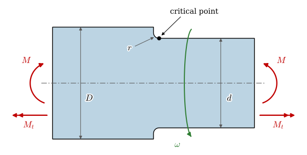
As the shaft turns, a point on its surface passes from the tension side to the compression side and back, so the bending stress is fully reversed, while the torque gives a constant shear stress. With the nominal stresses of 8.19.5,
\[ \sigma_a = \frac{32M}{\pi d^3}, \quad \sigma_m = 0, \qquad \tau_a = 0, \quad \tau_m = \frac{16M_t}{\pi d^3} \]
The notch factors follow from 8.19.8, \(K_f = 1 + q(K_t - 1)\) and \(K_{fs} = 1 + q_s(K_{ts} - 1)\), and 8.21.13 reduces to \(\sigma_a' = K_f\sigma_a\) and \(\sigma_m' = \sqrt{3}K_{fs}\tau_m\). The endurance limit of the shaft is 8.21.9 with \(\sigma_e' = 0.5R_m\) from 8.21.5, the machined surface factor \(k_a = 4.51R_m^{-0.265}\), the size factor \(k_b = 1.24d^{-0.107}\) and all other factors equal to one, for a median life. The factor of safety follows from 8.21.11, and the first-cycle check against yielding from the largest von Mises stress, \(\sigma_{\max}' = \sqrt{(K_f\sigma_a)^2 + 3(K_{fs}\tau_m)^2}\).
d_s, M, M_t = 32, 200e3, 300e3             # mm, N mm, N mm, so stresses in MPa
R_m, R_p = 700, 500
K_t, K_ts, q, q_s = 1.88, 1.51, 0.82, 0.86

sigma_a = 32*M/(np.pi*d_s**3)
tau_m = 16*M_t/(np.pi*d_s**3)
K_f, K_fs = 1 + q*(K_t - 1), 1 + q_s*(K_ts - 1)                  # @eq-kf
sa_vm, sm_vm = K_f*sigma_a, np.sqrt(3)*K_fs*tau_m               # @eq-fatigue-von-mises

k_a, k_b = 4.51*R_m**-0.265, 1.24*d_s**-0.107
sigma_e = k_a*k_b*0.5*R_m                                       # @eq-marin

n_fatigue = 1/(sa_vm/sigma_e + sm_vm/R_m)                       # @eq-goodman
n_yield = R_p/np.sqrt(sa_vm**2 + sm_vm**2)

ltx(r"K_f &=", K_f, r", \quad K_{fs} =", K_fs,
    r", \quad \sigma_a' =", sa_vm, r"~\text{MPa}, \quad \sigma_m' =", sm_vm, r"~\text{MPa}",
    r"\\ k_a &=", k_a, r", \quad k_b =", k_b, r", \quad \sigma_e =", sigma_e, r"~\text{MPa}",
    r"\\ n &=", n_fatigue, r", \quad n_y =", n_yield,
    aligned=True, precision=3)
\[ \begin{aligned}K_f &=1.72, \quad K_{fs} =1.44, \quad \sigma_a' =107.0~\text{MPa}, \quad \sigma_m' =116.0~\text{MPa}\\ k_a &=0.795, \quad k_b =0.856, \quad \sigma_e =238.0~\text{MPa}\\ n &=1.62, \quad n_y =3.17\end{aligned} \]
The surface and the size together reduce the endurance limit from \(350\) to \(238~\text{MPa}\), and the shoulder raises the bending amplitude from \(62\) to \(107~\text{MPa}\). The factor of safety against fatigue is about \(1.6\), half the static factor of safety of the same shaft. The point \((\sigma_m', \sigma_a')\) lies inside the Goodman line in Figure 8.21.20, and the shaft has an infinite life.
If the bending moment doubles, the amplitude doubles while the mean stays. 8.21.12 converts the cycle to an equally damaging fully reversed one, and if that lies above the endurance limit, the line of 8.21.6 with \(f = 0.85\) and 8.21.7 give the life,
\[ \sigma_{ar} = \frac{2\sigma_a'}{1 - \sigma_m'/R_m}, \qquad N = \left(\frac{\sigma_{ar}}{a}\right)^{1/b} \]
and at \(n_r\) revolutions per minute the shaft completes them in \(t = N/(60\,n_r)\) hours.
Code
sa_over = 2*sa_vm
s_ar = sa_over/(1 - sm_vm/R_m)                                  # @eq-equivalent-amplitude
a_sn = (f_sn*R_m)**2/sigma_e                                    # @eq-basquin-constants
b_sn = -np.log10(f_sn*R_m/sigma_e)/3
N_over = (s_ar/a_sn)**(1/b_sn)                                  # @eq-life
n_r = 1000                                                      # rpm
t_over = N_over/(60*n_r)                                        # h

ltx(r"\sigma_{ar} =", s_ar, r"~\text{MPa}, \quad a =", a_sn, r"~\text{MPa}, \quad b =", b_sn,
    r", \quad N =", N_over/1e5, r"\cdot 10^5, \quad t =", t_over, r"~\text{h}", precision=3)
\[ \sigma_{ar} =257.0~\text{MPa}, \quad a =1.49 \cdot 10^{3}~\text{MPa}, \quad b =-0.133, \quad N =5.67\cdot 10^5, \quad t =9.45~\text{h} \]
The doubled moment gives a life of about \(5.7 \cdot 10^5\) revolutions, under ten hours of running. Since the endurance limit is exceeded by only \(8~\%\), the life is sensitive to every number in the calculation, and the result should be read as an order of magnitude.
If the doubled moment acts only during \(5~\%\) of the revolutions, the remaining \(95~\%\) lie below the endurance limit and, by 8.21.14, cause no damage. A total of \(N_{\text{tot}}\) revolutions then gives the damage \(D = 0.05\,N_{\text{tot}}/N\), and the shaft lasts
\[ N_{\text{tot}} = \frac{N}{0.05}, \qquad t_{\text{tot}} = \frac{N_{\text{tot}}}{60\,n_r} \]
Code
N_tot = N_over/0.05
ltx(r"N_{\text{tot}} =", N_tot/1e7, r"\cdot 10^7, \quad t_{\text{tot}} =", N_tot/(60*n_r), r"~\text{h}",
    precision=3)
\[ N_{\text{tot}} =1.13\cdot 10^7, \quad t_{\text{tot}} =189.0~\text{h} \]
The shaft lasts about \(1.1 \cdot 10^7\) revolutions, or \(190\) hours. The reservations of the previous section apply with force here: once the overloads have started a crack, the normal cycles grow it too, and the true life may be considerably shorter. Figure 8.21.20 collects the two load cycles of Example 1 in the Haigh diagram.
Code
sm = np.linspace(0, R_m, 200)

fig, ax = plt.subplots(figsize=(6, 4.0))
ax.plot([0, R_m], [sigma_e, 0], color='C0', lw=2, label='Goodman')
ax.plot(sm, sigma_e*(1 - (sm/R_m)**2), color='C2', lw=1.5, ls='--', label='Gerber')
ax.plot([0, R_p], [sigma_e, 0], color='C4', lw=1.5, ls='-.', label='Soderberg')
ax.plot([0, R_p], [R_p, 0], color='C3', lw=1.5, ls=':', label='Langer (yield)')
ax.plot([0, 3*sm_vm], [0, 3*sa_vm], color='0.35', lw=0.8)
ax.plot(sm_vm, sa_vm, 'o', color='black', ms=6, label=f'$M = 200$ N m, $n = {n_fatigue:.2f}$')
ax.plot(sm_vm, sa_over, 's', color='C3', ms=6, label='$M = 400$ N m')
ax.set_xlabel(r"mean stress $\sigma_m'$ [MPa]")
ax.set_ylabel(r"stress amplitude $\sigma_a'$ [MPa]")
ax.set_xticks([0, 116, 500, 700])
ax.set_yticks([0, 107, 214, 238, 500])
ax.set_xlim(0, R_m)
ax.set_ylim(0, 520)
ax.grid(True, alpha=0.4)
ax.legend(fontsize=9)
plt.show()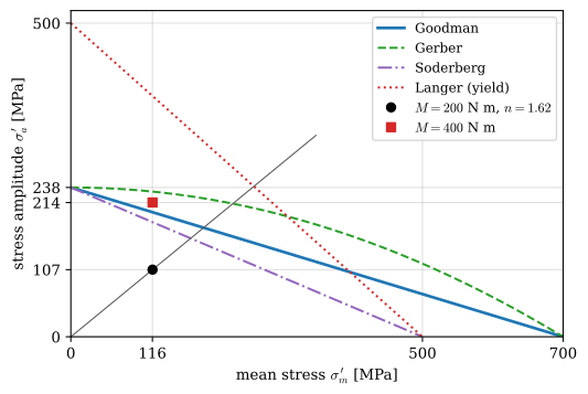
The example shows where the design leverage lies. A fillet radius of \(4~\text{mm}\) would lower \(K_t\) and with it the amplitude, a ground surface would raise \(k_a\) from \(0.80\) to about \(0.91\), and both act on the term \(\sigma_a'/\sigma_e\) that dominates 8.21.11, while a stronger steel helps less than its tensile strength suggests, because \(k_a\) falls as \(R_m\) rises.
Designing against fatigue
The rules that follow from this chapter are few. Keep the stress amplitude low where the stress concentrations are, which means generous fillet radii and discontinuities placed where the nominal stress is small, as Chapter 8.19 recommends. Make the surface at the critical points smooth, since cracks start at the surface. Introduce compressive residual stresses there, by shot peening, by rolling the fillets and threads, or by surface hardening, since a compressive mean stress closes cracks. Avoid welding or attaching anything to a highly stressed member: a weld toe is a sharp notch with tensile residual stresses, and the Kielland platform failed from a small fillet weld on a member that carried the main loads. Where cyclic loads cannot be avoided, use a material with an endurance limit, and for an aluminium part, which has none, design for a finite and stated life.
For 3D-printed polymer parts no endurance limit can be assumed, and the boundaries between layers act as built-in notches. A cyclic tension that pulls the layers apart is the most damaging, so a part loaded repeatedly should be oriented on the print bed so that the main stresses run along the layers, and its fillets should be rounded as generously as for a metal part. Published fatigue data for printed parts depend strongly on the material and the print settings, and a part that matters should be tested.
The finite element method delivers the stress field from which a fatigue check starts. Fatigue post-processors take the stresses of each load case, or a measured or simulated load history, and apply the methods of this chapter point by point: they count the cycles, compute amplitudes and means, correct for the surface and the mean stress, and sum the damage with 8.21.14. They inherit the scatter of the material data, and their result is an estimate of the life, not a guarantee.
A crack that has already been found falls outside the S-N curve, whose lives include the initiation that has already happened, and it is assessed with fracture mechanics. The stress field at the tip of a crack of length \(a\) under the nominal stress \(\sigma\) is scaled by the stress intensity factor \(K = Y\sigma\sqrt{\pi a}\), where the factor \(Y\) depends on the geometry of the part and the crack. The part breaks when \(K\) reaches the fracture toughness \(K_{Ic}\) of the material, which fixes a critical crack length \(a_c\). Below it the crack grows on every cycle by an amount that Paris and Erdogan found to depend on the range \(\Delta K = Y\Delta\sigma\sqrt{\pi a}\) alone [15],
\[ \frac{da}{dN} = C\,\Delta K^{m} \]
with the material constants \(C\) and \(m\), where \(m\) is about three for steels. Integrating from the crack that was found, \(a_0\), to \(a_c\) gives the cycles left, and since a short crack grows slowly, most of them are spent while the crack is still small. For a constant \(Y\) the integral gives a life proportional to \(\Delta\sigma^{-m}\), an S-N line of slope \(m \approx 3\), the slope of the design curves for welded joints, whose life is almost all crack growth. The same calculation sets the inspection intervals of aircraft structures, so that a crack too small to be found at one inspection cannot reach \(a_c\) before the next. The wheels at Eschede were inspected by eye, which finds only a long crack. Fracture mechanics is a subject of its own [16].
Further reading
Shigley’s chapter on fatigue failure covers the stress-life method of this chapter in full, including the charts for the notch sensitivity and many worked examples of shafts [5]. DNV-RP-C203 is free to download and shows how a design code turns the methods of this chapter into rules for welded structures [6].
References
[1]
Wöhler A. Über die festigkeits-versuche mit eisen und stahl. Zeitschrift Für Bauwesen 1870;20:73–106.
[2]
Manson SS. Behavior of materials under conditions of thermal stress. Washington, DC: National Advisory Committee for Aeronautics; 1953.
[3]
Coffin, Jr. LF. A study of the effects of cyclic thermal stresses on a ductile metal. Transactions of the American Society of Mechanical Engineers 1954;76:931–50.
[4]
Basquin OH. The exponential law of endurance tests. Proceedings of the American Society for Testing and Materials 1910;10:625–30.
[5]
Budynas RG, Nisbett JK. Shigley’s mechanical engineering design. 11th ed. New York: McGraw-Hill Education; 2020.
[6]
DNV-RP-C203 Fatigue design of offshore steel structures. Høvik, Norway: DNV; 2021.
[7]
BS 7608:2014+A1:2015 Guide to fatigue design and assessment of steel products. London: British Standards Institution; 2015.
[8]
EN 1993-1-9:2005 Eurocode 3: Design of steel structures – Part 1-9: Fatigue. Brussels: European Committee for Standardization; 2005.
[9]
Björk K. Formler och tabeller för mekanisk konstruktion. 9th ed. Spånga: Karl Björks förlag HB; 2022.
[10]
Goodman J. Mechanics applied to engineering. London: Longmans, Green; Co.; 1899.
[11]
Palmgren A. Die lebensdauer von kugellagern. Zeitschrift Des Vereines Deutscher Ingenieure 1924;68:339–41.
[12]
Miner MA. Cumulative damage in fatigue. Journal of Applied Mechanics 1945;12:A159–64.
[13]
Matsuishi M, Endo T. Fatigue of metals subjected to varying stress. Proceedings of the kyushu district meeting of the japan society of mechanical engineers, Fukuoka: 1968, p. 37–40.
[14]
ASTM E1049-85 (Reapproved 2017) Standard Practices for Cycle Counting in Fatigue Analysis. West Conshohocken, PA: ASTM International; 2017. https://doi.org/10.1520/E1049-85R17.
[15]
Paris PC, Erdogan F. A critical analysis of crack propagation laws. Journal of Basic Engineering 1963;85:528–33. https://doi.org/10.1115/1.3656900.
[16]
Anderson TL. Fracture mechanics: Fundamentals and applications. 4th ed. Boca Raton, FL: CRC Press; 2017. https://doi.org/10.1201/9781315370293.