In Chapter 8.7 the stress at a point became a tensor, and Cauchy’s formula 8.7.9 gave the traction on any cut through the point. Turning the cut changes the normal and the shear stress on it, and in 1882 the German engineer Otto Mohr1 showed that in a plane the pair of them traces a circle [1]. Karl Culmann had drawn such circles for the stresses in a beam some fifteen years earlier, and Mohr made the construction general.
The circle holds a whole stress state in one picture. Every cut through the point is a point on the circle, the principal stresses are where the circle crosses the axis, and the largest shear stress is its radius. Many textbooks teach the circle as a graphical method of calculation, drawn with ruler and compass. We leave the calculation to the eigenvalue problem 8.7.10 and a few lines of code, and use the circle to see why the results come out as they do: why a ductile bar in tension slips on planes at \(45^\circ\), why a hydrostatic stress has no shear on any plane, why the Tresca criterion ignores the intermediate principal stress and why a hydrostatic pressure does not make a metal yield.
From the rotated cut to a circle
We start from the bar in uniaxial tension of Example 2 in the chapter on shear stress, cut at the angle \(\varphi\) to its axis. With \(\sigma_0 = P/A\), 8.4.2 gives \(\sigma_\varphi = \sigma_0\sin^2\varphi\) and \(\tau_\varphi = \sigma_0\sin\varphi\cos\varphi\). The double-angle identities \(\sin^2\varphi = \tfrac{1}{2}(1 - \cos 2\varphi)\) and \(\sin\varphi\cos\varphi = \tfrac{1}{2}\sin 2\varphi\) turn the pair into
As the cut turns, the point \((\sigma_\varphi, \tau_\varphi)\) moves on a circle with its centre at \(\sigma_0/2\) on the \(\sigma\) axis and the radius \(\sigma_0/2\). The circle passes through the origin, the cut along the bar, which carries no stress, and through \(\sigma_0\), the cross-section. The angle appears doubled. Turning the cut through \(90^\circ\), from along the bar to across it, carries the point half way round the circle, and turning it through \(180^\circ\) brings the point back to where it started, as it must, since a plane turned half a turn is the same plane.
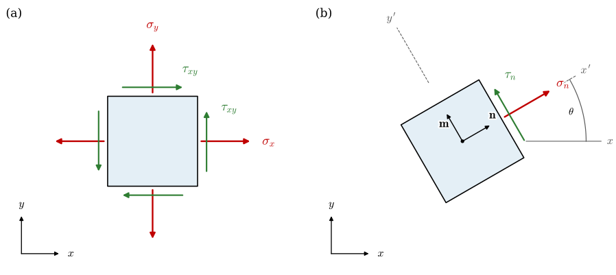
The same happens for any plane stress state. Figure 8.8.1 (a) shows the element with the stresses \(\sigma_x\), \(\sigma_y\) and \(\tau_{xy}\), all drawn positive. A cut whose unit normal makes the angle \(\theta\) with the \(x\) axis, counted counterclockwise, has the normal and tangent
\[
\bm n = [\cos\theta, \sin\theta]^\mathsf{T}, \qquad \bm m = [-\sin\theta, \cos\theta]^\mathsf{T}
\]
where \(\bm m\) is \(\bm n\) turned \(90^\circ\) counterclockwise, the same choice as in Example 1 of the chapter on stress and strain states, which reproduced 8.4.2. The normal stress \(\sigma_n\) and the shear stress \(\tau_n\) on the cut are the components of the traction \(\bm t = \bm\sigma\bm n\) along \(\bm n\) and \(\bm m\), Figure 8.8.1 (b).
Figure 8.8.1: (a) A plane stress element with \(\sigma_x\), \(\sigma_y\) and \(\tau_{xy}\) drawn positive. (b) A cut through the same point whose normal \(\bm n\) makes the angle \(\theta\) with the \(x\) axis, and the normal stress \(\sigma_n\) along \(\bm n\) and the shear stress \(\tau_n\) along \(\bm m\), \(\bm n\) turned counterclockwise. Both are drawn positive: \(\tau_n > 0\) is a shear stress that would turn the element counterclockwise.
Multiplying out \(\sigma_n = \bm n^\mathsf{T}\bm\sigma\bm n\) and \(\tau_n = \bm m^\mathsf{T}\bm\sigma\bm n\) and using the double-angle identities once more gives
We move the constant term of the first line to the left, square both lines and add them. The cross terms cancel, \(\cos^2 2\theta + \sin^2 2\theta = 1\) removes the angle, and what remains is
Every cut through the point is therefore a point on one circle, Mohr’s circle, with its centre \(c\) on the \(\sigma\) axis and the radius \(R\). The centre is half the trace of the stress tensor, and \(R^2 = c^2 - \det\bm\sigma\), so both are the same in every frame, as the coefficients of 8.7.11 were. The frame we start in decides only where on the circle the \(x\) face lies. SymPy confirms both steps, from Cauchy’s formula to 8.8.2 and from there to the circle.
At \(\theta = 0\) the cut is the \(x\) face of the element, and 8.8.2 gives the point \((\sigma_x, \tau_{xy})\). At \(\theta = 90^\circ\) it is the \(y\) face, where \(\bm n = \bm e_y\) and \(\bm m = -\bm e_x\), and the point is \((\sigma_y, -\tau_{xy})\). The two points lie at the ends of a diameter, and so do any two faces of an element at right angles to each other, since \(90^\circ\) on the element is \(180^\circ\) on the circle.
The circle crosses the \(\sigma\) axis at \(c \pm R\), which is 8.7.12: the principal stresses are the cuts that carry no shear stress. As in Principal stresses in three dimensions, the two in-plane principal stresses are written \(\sigma_\text{I} \geq \sigma_\text{II}\), which leaves the indices \(1\), \(2\), \(3\) for ordering all three principal stresses of a point, out of the plane included, in the section on three dimensions. The highest and lowest points of the circle are the cuts with the largest shear stress in the plane,
\[
\tau_{\max} = R = \frac{\sigma_\text{I} - \sigma_\text{II}}{2}
\]
a quarter turn round the circle from the principal points, and therefore at \(45^\circ\) to the principal directions on the element. The normal stress on those cuts is \(c\), which is zero only when \(\sigma_x + \sigma_y = 0\).
Which way the point turns
The direction of travel follows from writing \(\tfrac{1}{2}(\sigma_x - \sigma_y) = R\cos 2\theta_p\) and \(\tau_{xy} = R\sin 2\theta_p\). Then 8.8.2 reads
At \(\theta = \theta_p\) the shear stress vanishes and \(\sigma_n = c + R = \sigma_\text{I}\), so \(\theta_p\) is the principal angle, the angle from the \(x\) axis to the direction of \(\sigma_\text{I}\),
with \(2\theta_p\) taken in the quadrant where \(\cos 2\theta_p\) has the sign of \(\sigma_x - \sigma_y\) and \(\sin 2\theta_p\) the sign of \(\tau_{xy}\), as the two-argument arctangent does. The minus sign in front of the sine means that the point turns clockwise in a plot with \(\tau_n\) upward while the cut turns counterclockwise. We therefore draw the \(\tau_n\) axis positive downward, as many textbooks do. The rule is then the same on both sides: turning the element counterclockwise through \(\theta\) turns its point counterclockwise through \(2\theta\). A face whose shear stress would turn the element counterclockwise, as \(\tau_n\) in Figure 8.8.1 (b) would, lies below the \(\sigma\) axis.
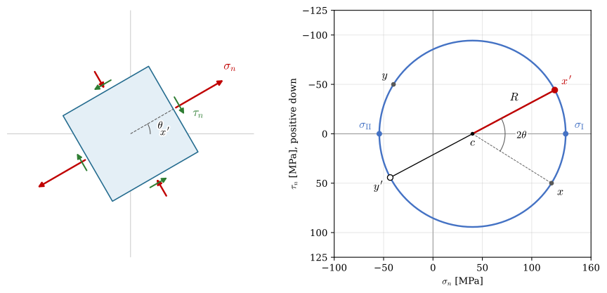
Figure 8.8.2: The state of Example 2 turned through \(\theta = 30^\circ\). Left, the element with the normal stresses (red) and shear stresses (green) on its faces, drawn to scale. Right, Mohr’s circle with \(\tau_n\) positive downward. The grey points \(x\) and \(y\) are the faces of the unturned element, the red point \(x'\) and the open point \(y'\) those of the turned one, at the ends of a diameter. Turning the element counterclockwise through \(\theta\) turns the radius to \(x'\) counterclockwise through \(2\theta\). The blue points are the principal stresses \(\sigma_\text{I}\) and \(\sigma_\text{II}\).
The numbers behind the figure follow from 8.8.2 at \(\theta = 30^\circ\) and at \(\theta = 120^\circ\) for the two faces, from 8.8.3 for the circle and from 8.8.4 for the principal angle.
The face \(x'\) carries a tensile stress of \(123~\text{MPa}\) and a shear stress of \(-44~\text{MPa}\), which turns the element clockwise and puts the point above the axis. The two faces carry shear stresses of equal size and opposite sign, as opposite points of the circle must, and their normal stresses add up to \(2c = \sigma_x + \sigma_y = 80~\text{MPa}\) at every angle. The principal stresses \(134~\text{MPa}\) and \(-54~\text{MPa}\) and the principal angle \(16^\circ\) are those that Example 2 found from the eigenvalue problem.
Turning the element
The simulation below draws the element and its circle for any plane stress state, from 8.8.2 and 8.8.3 with \(\tau_n\) positive downward. The sliders set \(\sigma_x\), \(\sigma_y\), \(\tau_{xy}\) and the angle \(\theta\) through which the element is turned. The buttons turn the element to the principal angle 8.8.4, where the shear stress vanishes on every face, or \(45^\circ\) further on, to the largest shear stress, and the checkboxes load four states that the next section discusses. Below the controls the simulation reports the stresses on the faces \(x'\) and \(y'\), the principal stresses, the principal angle, and the largest shear stress both in the plane and over all planes through the point, the latter with \(\sigma_z = 0\) as the section on three dimensions explains.
Turning \(\theta\) slowly from \(0\) to \(90^\circ\) shows the face \(x'\) travel half way round the circle and arrive where \(y\) started. Raising \(\tau_{xy}\) with \(\sigma_x\) and \(\sigma_y\) fixed leaves the centre in place and swells the circle, and changing \(\sigma_x\) and \(\sigma_y\) by the same amount slides the circle along the axis without changing its size.
Reading stress states from the circle
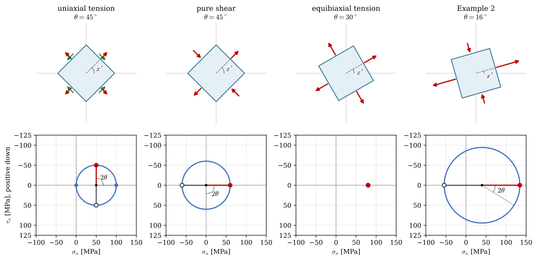
Four states recur throughout the book, and Figure 8.8.3 draws each of them with its element turned to the angle that tells the most.
Figure 8.8.3: Four plane stress states, each element turned to the angle named above it, and its circle with the face \(x'\) in red. Uniaxial tension \(\sigma = 100~\text{MPa}\): the circle passes through the origin and the largest shear stress, half the tension, acts at \(45^\circ\). Pure shear \(\tau = 60~\text{MPa}\): the circle is centred on the origin and at \(45^\circ\) the faces carry the principal stresses \(\pm\tau\). Equibiaxial tension \(80~\text{MPa}\): the circle shrinks to a point, and every face carries the same normal stress and no shear. Example 2 at its principal angle of \(16^\circ\).
In uniaxial tension\(\sigma\) the circle runs from the origin to \(\sigma\), as 8.8.1 found. Its lowest and highest points lie at a quarter turn from both ends, so the largest shear stress, \(\sigma/2\), acts on the planes at \(45^\circ\) to the load, together with the normal stress \(\sigma/2\). Plastic slip in a metal is driven by shear, and a ductile tensile specimen yields first along bands at about \(45^\circ\) to its axis, as the chapter on shear stress observed.
In pure shear\(\sigma_x = \sigma_y = 0\), the centre \(c\) is zero and the circle is centred on the origin with the radius \(\tau\). A quarter turn round it lie the principal stresses \(\sigma_\text{I} = \tau\) and \(\sigma_\text{II} = -\tau\), on planes at \(45^\circ\) to the shear: pure shear is an equal tension and compression at right angles. The surface of a twisted shaft is in this state, and a stick of chalk twisted between the fingers breaks along a helix at \(45^\circ\) to its axis, perpendicular to \(\sigma_\text{I}\), since a brittle material opens where the tension is largest, as Figure 8.10.1 shows.
In equibiaxial tension\(\sigma_x = \sigma_y\) and \(\tau_{xy} = 0\), the radius is zero and the circle is a single point. Every cut in the plane carries the same normal stress and no shear stress, and every direction in the plane is a principal direction. When the third normal stress is equal too, the state is hydrostatic, the pressure in a fluid, and the three circles of the next section collapse onto one point: there is no shear stress on any plane through the point, whatever its orientation.
A general state such as Example 2 has a circle that straddles the origin, and so one tensile and one compressive principal stress, or lies to one side of it, with two of the same sign. Where the circle lies is set by the mean of the normal stresses, how large it is by their difference and by the shear stress.
Three dimensions: three circles
A general state has three principal stresses, the eigenvalues of the \(3 \times 3\) stress tensor, ordered
\[
\sigma_1 \geq \sigma_2 \geq \sigma_3
\]
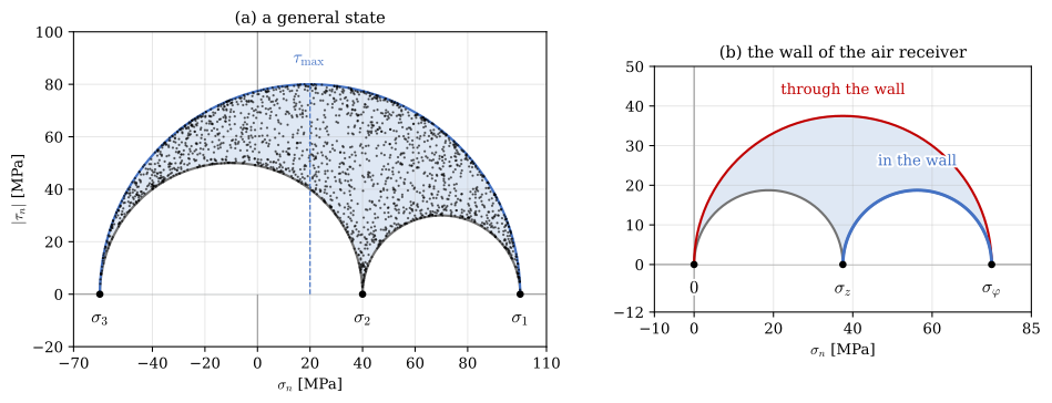
so that \(\sigma_2\) is the intermediate one. In the principal frame a cut whose normal is perpendicular to one principal direction sees only the other two, and 8.8.3 applies to it with those two in place of \(\sigma_x\) and \(\sigma_y\). Such cuts fill three circles, through \(\sigma_1\) and \(\sigma_2\), through \(\sigma_2\) and \(\sigma_3\), and through \(\sigma_1\) and \(\sigma_3\). Mohr showed that every other cut through the point lands in the region between them: inside the largest circle and outside the two smaller ones [1]. In three dimensions the shear stress on a cut is a vector in the plane of the cut with no preferred direction, so we plot its magnitude \(|\tau_n|\), above the axis, and draw the upper half of each circle.
The largest circle sets the largest shear stress over all planes,
which is 8.7.14, and it acts on the planes at \(45^\circ\) between the directions of \(\sigma_1\) and \(\sigma_3\). Figure 8.8.4 (a) checks the claim about the region for the state \(\sigma_1 = 100\), \(\sigma_2 = 40\) and \(\sigma_3 = -60~\text{MPa}\). With the normal \(\bm n = [n_1, n_2, n_3]^\mathsf{T}\) in the principal frame, Cauchy’s formula gives \(\bm t = [\sigma_1 n_1, \sigma_2 n_2, \sigma_3 n_3]^\mathsf{T}\), and the stresses on the cut are
which we evaluate for two thousand random normals.
Plane stress needs one more thought. A free surface carries no stress, so \(\sigma_z = 0\) is a principal stress, and the three principal stresses are \(\sigma_\text{I}\), \(\sigma_\text{II}\) and \(0\), sorted. When the in-plane principal stresses have opposite signs, as in Example 2, the zero lies between them, the in-plane circle is the largest of the three, and \(\tau_{\max} = R\). When both have the same sign, the zero is \(\sigma_3\) or \(\sigma_1\) and the largest circle is one through the origin. The wall of the compressed-air receiver in Example 2 of the chapter on yield criteria is such a case, with the hoop stress \(\sigma_\varphi = 75~\text{MPa}\), the axial stress \(\sigma_z = 37.5~\text{MPa}\) and no stress normal to its outer surface. Figure 8.8.4 (b) shows that the in-plane circle, between \(37.5\) and \(75~\text{MPa}\), has the radius \(18.75~\text{MPa}\), while the largest shear stress at the point is \(37.5~\text{MPa}\), on planes at \(45^\circ\) through the wall thickness. A check confined to the plane of the wall would understate it by a factor of two.
Code
def three_circles(ax, s, colors=('0.45', '0.45', BLUE), shade='#dfe8f4', lw=1.6, ls='-'):"""The upper halves of the three circles of the principal stresses s, region shaded.""" s1, s2, s3 =sorted(s, reverse=True) a = np.linspace(0, np.pi, 181) pairs = [(s1, s2), (s2, s3), (s1, s3)]if shade: c, r = (s1 + s3)/2, (s1 - s3)/2 ax.fill(c + r*np.cos(a), r*np.sin(a), color=shade, zorder=1, lw=0)for p, q in pairs[:2]: ax.fill((p + q)/2+ (p - q)/2*np.cos(a), (p - q)/2*np.sin(a), color='white', zorder=1.5, lw=0)for (p, q), col inzip(pairs, colors): ax.plot((p + q)/2+ (p - q)/2*np.cos(a), (p - q)/2*np.sin(a), color=col, lw=lw, ls=ls, zorder=3) ax.plot([s1, s2, s3], [0, 0, 0], 'o', color='black', ms=4, zorder=5) ax.axhline(0, color='0.5', lw=0.7, zorder=0) ax.axvline(0, color='0.5', lw=0.7, zorder=0) ax.set_aspect('equal')def random_planes(s, N, seed=1):"""sigma_n and |tau_n| on N cuts with random normals, s the principal stresses.""" n = np.random.default_rng(seed).normal(size=(N, 3)) n /= np.linalg.norm(n, axis=1, keepdims=True) t = n*np.asarray(s, float) # Cauchy's formula in the principal frame sn = np.sum(t*n, axis=1)return sn, np.sqrt(np.maximum(np.sum(t*t, axis=1) - sn**2, 0))s_gen = (100, 40, -60)s_vessel = (75, 37.5, 0)fig, (ax, bx) = plt.subplots(1, 2, figsize=(10.5, 3.9), gridspec_kw={'width_ratios': [1.6, 1]})three_circles(ax, s_gen)sn, tn = random_planes(s_gen, 2000)ax.plot(sn, tn, '.', color='black', ms=1.5, alpha=0.55, zorder=4)for v, s inzip(s_gen, (r'$\sigma_1$', r'$\sigma_2$', r'$\sigma_3$')): text(ax, (v, -9), s, fs=12)text(ax, (20, 90), r'$\tau_{\max}$', BLUE, 12)ax.plot([20, 20], [0, 80], color=BLUE, lw=0.9, ls='--', zorder=4)ax.set_xlim(-70, 110)ax.set_ylim(-20, 100)ax.set_xlabel(r'$\sigma_n$[MPa]')ax.set_ylabel(r'$|\tau_n|$[MPa]')ax.set_title('(a) a general state', fontsize=11)three_circles(bx, s_vessel, colors=('0.45', '0.45', LOAD))a = np.linspace(0, np.pi, 91)bx.plot(56.25+18.75*np.cos(a), 18.75*np.sin(a), color=BLUE, lw=2.2, zorder=4)text(bx, (56.25, 26), 'in the wall', BLUE, 10)text(bx, (37.5, 44), 'through the wall', LOAD, 10)for v, s inzip(s_vessel, (r'$\sigma_\varphi$', r'$\sigma_z$', r'$0$')): text(bx, (v, -6), s, fs=12)bx.set_xlim(-10, 85)bx.set_ylim(-12, 50)bx.set_xlabel(r'$\sigma_n$[MPa]')bx.set_title('(b) the wall of the air receiver', fontsize=11)for q in (ax, bx): q.grid(True, alpha=0.3)fig.tight_layout()end_ticks(fig)plt.show()
Figure 8.8.4: The three circles of a three-dimensional state, drawn as their upper halves with the magnitude of the shear stress. (a) \(\sigma_1 = 100\), \(\sigma_2 = 40\) and \(\sigma_3 = -60~\text{MPa}\). Two thousand cuts with random normals (dots) all fall in the shaded region between the largest circle and the two smaller ones. (b) The outer surface of the air receiver wall. The in-plane circle (blue) has half the radius of the largest circle (red), which passes through the zero stress normal to the surface.
All two thousand cuts in (a) fall in the shaded region. Counting the ones that do not, with a small tolerance for round-off, confirms it.
Code
def outside(s, sn, tn, tol=1e-9):"""The number of cuts outside the region between the three circles.""" s1, s2, s3 =sorted(s, reverse=True) d =lambda p, q: (sn - (p + q)/2)**2+ tn**2- ((p - q)/2)**2# > 0 outside that circlereturnint(np.sum((d(s1, s3) > tol) | (d(s1, s2) <-tol) | (d(s2, s3) <-tol)))ltx(r"\text{cuts outside the region} =", outside(s_gen, sn, tn),r"\quad\text{of}\quad", len(sn))
\[ \text{cuts outside the region} =0\quad\text{of}\quad2000 \]
Mohr’s circle and yielding
The yield criteria of Chapter 8.10 reduce a stress state to an effective stress. Two of them read directly off the circles, and seeing them there explains their two most important properties.
Tresca: the size of the largest circle
The Tresca criterion 8.10.4 states that a ductile material yields when \(\sigma_1 - \sigma_3 = \sigma_\text{Y}\). The left-hand side is the diameter of the largest circle, and the right-hand side is the diameter of the circle of a tensile test at yield, which runs from \(0\) to \(\sigma_\text{Y}\). Tresca’s criterion is a statement about size alone: the material yields when its largest circle has grown as large as the circle of the tensile test at yield, wherever on the axis it lies.
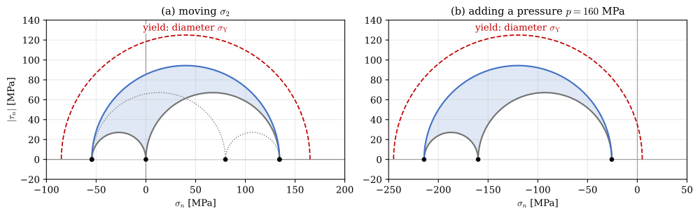
Two consequences can be seen at once. The intermediate principal stress \(\sigma_2\) only decides how the largest circle is split into the two smaller ones, and moving it between \(\sigma_3\) and \(\sigma_1\) leaves the largest circle as it is, so \(\sigma_2\) does not enter the criterion. And adding a hydrostatic pressure \(p\) to the state, \(\sigma_k \to \sigma_k - p\) for all three, slides all three circles along the axis by \(p\) without changing their sizes, so a hydrostatic pressure does not bring the material closer to yielding, however large it is. Figure 8.8.5 shows both for the principal stresses of Example 2, \(\sigma_1 = 134\), \(\sigma_2 = 0\) and \(\sigma_3 = -54~\text{MPa}\), with the yield strength \(\sigma_\text{Y} = 250~\text{MPa}\) of that example.
Code
sigma_Y =250.0s_ex2 = (c0 + R0, 0.0, c0 - R0)p_hyd =160.0a = np.linspace(0, np.pi, 181)fig, (ax, bx) = plt.subplots(1, 2, figsize=(10.5, 3.6))for q, s, title in ((ax, s_ex2, '(a) moving $\\sigma_2$'), (bx, tuple(v - p_hyd for v in s_ex2), '(b) adding a pressure $p = 160$ MPa')): three_circles(q, s) s1, s3 =max(s), min(s) cc = (s1 + s3)/2# the Tresca limit: diameter sigma_Y, same centre q.plot(cc + sigma_Y/2*np.cos(a), sigma_Y/2*np.sin(a), color=LOAD, lw=1.3, ls='--', zorder=3) q.set_title(title, fontsize=11) q.set_xlabel(r'$\sigma_n$[MPa]') q.grid(True, alpha=0.3)# in (a), sigma_2 moved to 80 MPa: the two small circles change, the largest does notthree_circles(ax, (s_ex2[0], 80.0, s_ex2[2]), colors=('0.45', '0.45', BLUE), shade=None, lw=1.0, ls=':')text(ax, (c0, 132), r'yield: diameter $\sigma_\mathrm{Y}$', LOAD, 10)text(bx, (c0 - p_hyd, 132), r'yield: diameter $\sigma_\mathrm{Y}$', LOAD, 10)ax.set_xlim(-100, 200)bx.set_xlim(-250, 50)for q in (ax, bx): q.set_ylim(-20, 140)ax.set_ylabel(r'$|\tau_n|$[MPa]')fig.tight_layout()end_ticks(fig)plt.show()
Figure 8.8.5: The Tresca criterion on the circles of Example 2. The dashed red circle has the diameter \(\sigma_\text{Y} = 250~\text{MPa}\) of a tensile test at yield and is drawn about the centre of the largest circle; the material yields when the largest circle grows to it. (a) Moving the intermediate stress from \(\sigma_2 = 0\) to \(80~\text{MPa}\) (dotted) changes the two smaller circles but not the largest one. (b) A hydrostatic pressure of \(160~\text{MPa}\) slides all three circles to the left without changing their sizes.
The yield criteria chapter found the same two properties from the formula 8.10.4. On the circles they need no algebra: the criterion measures a size, and neither \(\sigma_2\) nor a hydrostatic pressure changes the size of the largest circle.
Von Mises: all three circles
The von Mises effective stress 8.7.21 depends on all three differences of principal stresses, and each difference is the diameter of one circle. With the radii \(R_{12} = \tfrac{1}{2}(\sigma_1 - \sigma_2)\), \(R_{23} = \tfrac{1}{2}(\sigma_2 - \sigma_3)\) and \(R_{13} = \tfrac{1}{2}(\sigma_1 - \sigma_3)\) the criterion becomes
A hydrostatic pressure changes none of the three radii, so von Mises, like Tresca, is blind to it. Unlike Tresca, it sees \(\sigma_2\), through the split of the largest circle. The two smaller radii add up to the largest, \(R_{12} + R_{23} = R_{13}\), and for a fixed largest circle the sum of squares in 8.8.6 is smallest when the split is even, \(R_{12} = R_{23} = R_{13}/2\), which gives \(\sigma_\text{vM} = \sqrt{3}\,R_{13}\). It is largest when one of the small circles shrinks to a point, which gives \(\sigma_\text{vM} = 2R_{13} = \sigma_\text{T}\). Between these two limits lies the \(15.5~\%\) by which the two criteria can differ, 8.10.19, and the even split is the state, pure shear among others, where they differ most.
Brittle materials: the Coulomb–Mohr envelope
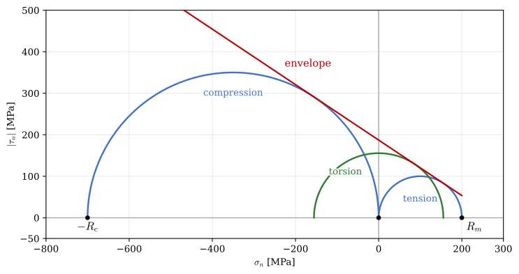
A brittle material such as grey cast iron is several times stronger in compression than in tension, and a criterion for it has to depend on where the circle lies, not only on its size. Mohr proposed to draw the circles of the states that cause failure in a few simple tests, the tensile test with the tensile strength \(R_m\) and the compression test with the compressive strength \(R_c\), and to draw the curve that touches them all, the failure envelope[2]. A state is safe while its largest circle stays inside the envelope and fails when the circle touches it. In the simplest version, after Coulomb’s law of friction, the envelope is the straight line tangent to the circles of the tensile and the compression test. That is the Coulomb–Mohr criterion[3,4].
The circles tangent to one straight line have radii that grow linearly with the position of their centres, \(r = \alpha + \beta c\). Fitting the line through the tensile test, \(c = r = R_m/2\), and the compression test, \(c = -R_c/2\) and \(r = R_c/2\), and requiring the largest circle of a state with \(\sigma_1 \geq 0 \geq \sigma_3\) to satisfy it, gives the criterion
which SymPy confirms. When both \(\sigma_1\) and \(\sigma_3\) are tensile the criterion is \(\sigma_1 = R_m\), and when both are compressive it is \(\sigma_3 = -R_c\), the tests themselves.
Code
R_m, R_c = sp.symbols('R_m R_c', positive=True)alpha, beta, cc = sp.symbols('alpha beta c', real=True)fit = sp.solve([sp.Eq(R_m/2, alpha + beta*R_m/2), # the tensile test circle sp.Eq(R_c/2, alpha + beta*(-R_c/2))], # the compression test circle [alpha, beta], dict=True)[0]# the largest circle of the state touches the envelope: its radius on the line r = alpha + beta ctouch = sp.Eq((s1 - s3)/2, (alpha + beta*(s1 + s3)/2).subs(fit))ltx(r"\alpha &=", sp.simplify(fit[alpha]), r",\quad \beta =", sp.simplify(fit[beta]),r"\\\frac{\sigma_1}{R_m} - \frac{\sigma_3}{R_c} &=", sp.simplify(sp.solve(touch, s1)[0]/R_m - s3/R_c), aligned=True)
The criterion follows the circles. In pure shear, \(\sigma_1 = \tau\) and \(\sigma_3 = -\tau\), 8.8.7 gives the shear strength \(\tau_f = R_m R_c/(R_m + R_c)\), which is the constant \(\alpha\) above and lies between \(R_m/2\) and \(R_m\). Figure 8.8.6 draws the envelope for a material with \(R_m = 200~\text{MPa}\) and \(R_c = 700~\text{MPa}\), of the order of a grey cast iron, with the torsion test circle that just touches it.
Code
Rm, Rc =200.0, 700.0tau_f = Rm*Rc/(Rm + Rc)bet = (Rm/2- Rc/2)/(Rm/2+ Rc/2) # the slope of r against cB = bet/np.sqrt(1- bet**2) # the envelope tau = A + B sigmaA = tau_f/np.sqrt(1- bet**2)a = np.linspace(0, np.pi, 181)fig, ax = plt.subplots(figsize=(8.6, 4.2))for cen, r, col, name, xy in ((Rm/2, Rm/2, BLUE, 'tension', (Rm/2, 45)), (-Rc/2, Rc/2, BLUE, 'compression', (-Rc/2, 300)), (0.0, tau_f, GREEN, 'torsion', (-80, 110))): ax.plot(cen + r*np.cos(a), r*np.sin(a), color=col, lw=1.8, zorder=3) text(ax, xy, name, col, 10)sg = np.linspace(-800, Rm, 2) # cut off at the tensile strengthax.plot(sg, A + B*sg, color=LOAD, lw=1.6, zorder=4)text(ax, (-170, A -170*B +70), 'envelope', LOAD, 11)ax.plot([-Rc, 0, Rm], [0, 0, 0], 'o', color='black', ms=4, zorder=5)text(ax, (Rm +30, -22), r'$R_m$', fs=12)text(ax, (-Rc, -22), r'$-R_c$', fs=12)ax.axhline(0, color='0.5', lw=0.7, zorder=0)ax.axvline(0, color='0.5', lw=0.7, zorder=0)ax.set_aspect('equal')ax.set_xlim(-800, 300)ax.set_ylim(-50, 500)ax.set_xlabel(r'$\sigma_n$[MPa]')ax.set_ylabel(r'$|\tau_n|$[MPa]')ax.grid(True, alpha=0.3)fig.tight_layout()end_ticks(fig)plt.show()
Figure 8.8.6: The Coulomb–Mohr envelope (red) of a brittle material with \(R_m = 200~\text{MPa}\) and \(R_c = 700~\text{MPa}\): the straight line tangent to the circles of the tensile and the compression test at failure. A state fails when its largest circle touches the line. The torsion circle that does is centred on the origin with the radius \(\tau_f = R_m R_c/(R_m + R_c) = 156~\text{MPa}\).
The envelope rises toward the compressive side. The further a circle lies to the left, the larger it may grow before it touches the line, and a compressive mean stress makes a brittle material stronger, the opposite of the ductile case, where position did not matter at all. Tests on cast iron follow this trend, and a modified form of the criterion that keeps \(\sigma_1 = R_m\) a little way into the region of a tensile and a compressive principal stress fits them better still [4].
Mohr’s circle for strain
The strain tensor transforms like the stress tensor, with the tensor shear strain \(\tfrac{1}{2}\gamma_{xy}\) in place of \(\tau_{xy}\). The normal strain \(\varepsilon_n\) and half the shear strain \(\tfrac{1}{2}\gamma_n\) in the direction at the angle \(\theta\) follow from 8.8.2 with \(\sigma \to \varepsilon\) and \(\tau \to \gamma/2\), and they lie on a circle with the centre \(\tfrac{1}{2}(\varepsilon_x + \varepsilon_y)\) and the radius of the square root in 8.7.13. The principal strains are where it crosses the \(\varepsilon\) axis. Plotting the full \(\gamma\) instead of \(\gamma/2\) would stretch the circle into an ellipse, which is the factor of two of the remark on tensor shear strain in the chapter on stress and strain states seen as a picture.
The strain circle is how strain gauge rosettes are read. A gauge measures only the normal strain along its own direction, and a rectangular rosette has three gauges at \(0^\circ\), \(45^\circ\) and \(90^\circ\). The gauges at \(0^\circ\) and \(90^\circ\) read \(\varepsilon_x\) and \(\varepsilon_y\), the two ends of a diameter, and the one at \(45^\circ\) reads the point a quarter turn round the circle, where 8.8.2 gives \(\varepsilon_{45} = \tfrac{1}{2}(\varepsilon_x + \varepsilon_y) + \tfrac{1}{2}\gamma_{xy}\). The shear strain, which no gauge measures, follows as
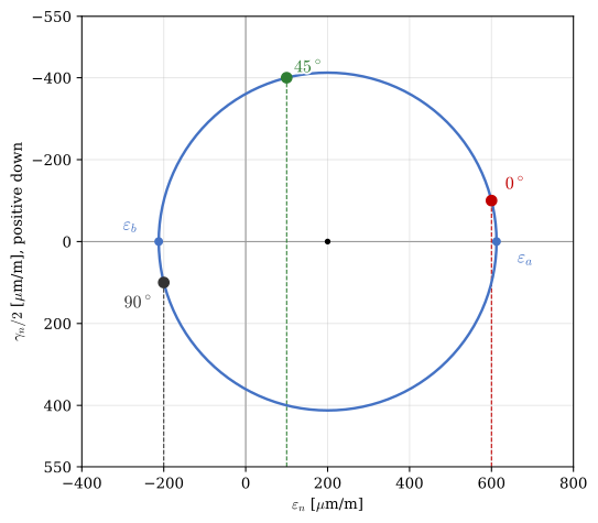
Figure 8.8.7 shows the three readings \(\varepsilon_0 = 600\), \(\varepsilon_{45} = 100\) and \(\varepsilon_{90} = -200~\mu\text{m/m}\) as three points of one circle.
Code
e0, e45, e90 =600.0, 100.0, -200.0# micrometres per metreg_half = e45 - (e0 + e90)/2# gamma_xy/2 from @eq-rosettece, Re = centre_radius(e0, e90, g_half) # the strain circle: tau -> gamma/2fig, ax = plt.subplots(figsize=(6.6, 5.0))draw_circle(ax, e0, e90, g_half, faces=False)for deg, col, d in ((0, LOAD, (60, -40)), (45, GREEN, (55, -25)), (90, '0.2', (-60, 50))): en, gn = on_cut(e0, e90, g_half, np.radians(deg)) ax.plot([en, en], [550, gn], color=col, lw=0.8, ls='--', zorder=2) ax.plot(en, gn, 'o', color=col, ms=7, zorder=6) text(ax, (en + d[0], gn + d[1]), rf'${deg}^\circ$', col, 12)text(ax, (ce + Re +70, 40), r'$\varepsilon_a$', BLUE, 12)text(ax, (ce - Re -70, -40), r'$\varepsilon_b$', BLUE, 12)ax.set_xlim(-400, 800)ax.set_ylim(550, -550)ax.set_xlabel(r'$\varepsilon_n$[$\mu$m/m]')ax.set_ylabel(r'$\gamma_n/2$[$\mu$m/m], positive down')ax.grid(True, alpha=0.3)fig.tight_layout()end_ticks(fig)plt.show()
Figure 8.8.7: Mohr’s circle for strain from a rectangular rosette. Each gauge reads the horizontal position of one point, dashed down to the axis. The \(0^\circ\) and \(90^\circ\) gauges lie opposite each other, the \(45^\circ\) gauge half way between them, and the three readings fix the circle and with it the principal strains \(\varepsilon_a\) and \(\varepsilon_b\).
From 8.8.8 and 8.7.13 the readings give the shear strain, the principal strains and, by 8.8.4 with strains, the principal angle.
Code
ltx(r"\gamma_{xy} &=", 2*g_half, r"~\mu\text{m/m}",r"\\\varepsilon_a &=", ce + Re, r"~\mu\text{m/m}, \quad \varepsilon_b =", ce - Re,r"~\mu\text{m/m}, \quad \theta_p =", np.degrees(0.5*np.arctan2(g_half, (e0 - e90)/2)), r"^\circ", aligned=True, precision=4)
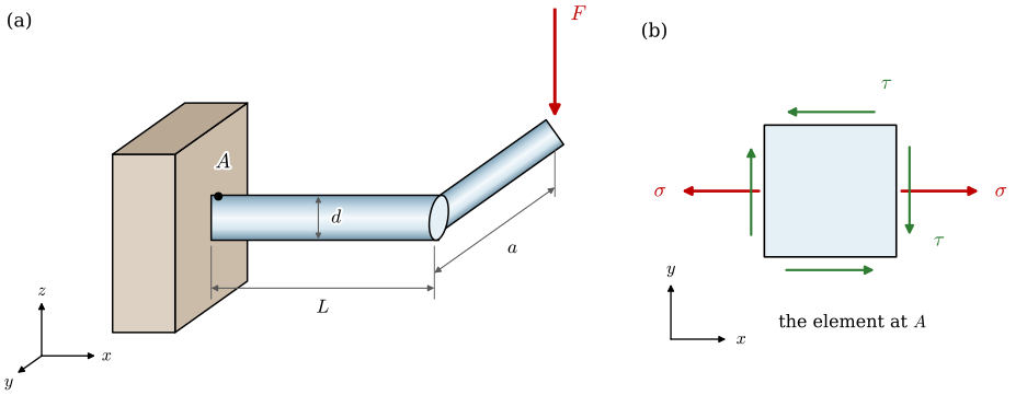
The crank shaft of Example 1 in the chapter on yield criteria, Figure 8.8.8, has the diameter \(d = 30~\text{mm}\) and is loaded by a force \(F = 1.5~\text{kN}\) at the end of an arm \(a = 300~\text{mm}\) long, whose plane lies \(L = 250~\text{mm}\) from the clamp. At the critical point \(A\) on top of the shaft at the clamp, the bending moment \(M = FL\) gives the normal stress \(\sigma = 32M/(\pi d^3)\) along the shaft and the torque \(M_t = Fa\) the shear stress \(\tau = 16M_t/(\pi d^3)\). The shaft is made of S355 with \(\sigma_\text{Y} = 355~\text{MPa}\). Draw the circles of the state at \(A\), follow them as the torque grows while the bending moment stays the same, and read off how far the torque can grow before \(A\) yields by Tresca’s criterion. Why does the maximum normal stress criterion give a misleading answer here?
Figure 8.8.8: (a) The shaft clamped at one end, with a crank arm of length \(a\) at the distance \(L\) from the clamp and a force \(F\) at the end of the arm. (b) The stress element at the critical point \(A\) on top of the shaft at the clamp, seen from above, with the bending stress \(\sigma\) and the torsional shear stress \(\tau\).
With \(x\) along the shaft as in Figure 8.8.8 (b), the state at \(A\) is \(\sigma_x = \sigma\), \(\sigma_y = 0\) and \(\tau_{xy} = -\tau\), since the shear stress on the \(+x\) face points along \(-y\). 8.8.3 gives the circle
\[
c = \frac{\sigma}{2}, \qquad R = \sqrt{\left(\frac{\sigma}{2}\right)^2 + \tau^2}
\]
with the \(x\) face at \((\sigma, -\tau)\) and the \(y\) face at \((0, \tau)\), on the \(\tau_n\) axis. Since \(R > c\) whenever \(\tau \neq 0\), the circle encloses the origin, so \(\sigma_\text{I} = c + R\) is tensile, \(\sigma_\text{II} = c - R\) compressive, and the zero normal to the surface lies between them:
\[
\sigma_1 = c + R, \qquad \sigma_2 = 0, \qquad \sigma_3 = c - R
\]
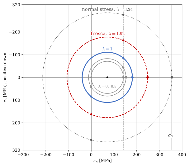
The in-plane circle is the largest of the three, and Tresca’s effective stress is its diameter, \(\sigma_\text{T} = 2R = \sqrt{\sigma^2 + 4\tau^2}\), 8.10.20. A growing torque, \(\tau \to \lambda\tau\) with the bending moment fixed, leaves the centre where it is and moves the \(x\) point straight up the line \(\sigma_n = \sigma\), so the circle swells about a fixed centre. Tresca’s criterion is reached when the diameter equals \(\sigma_\text{Y}\),
The maximum normal stress criterion compares only the right end of the circle, \(\sigma_1 = c + R\), with \(\sigma_\text{Y}\). Setting \(R = \sigma_\text{Y} - c\) gives \(\lambda^2\tau^2 = (\sigma_\text{Y} - c)^2 - c^2\), or
At the working load the circle has its centre at \(70.7~\text{MPa}\) and the radius \(110.5~\text{MPa}\), so \(\sigma_1 = 181~\text{MPa}\) and \(\sigma_3 = -40~\text{MPa}\). Figure 8.8.9 draws the circles as the torque grows.
Figure 8.8.9: The circles of the point \(A\) as the torque grows by the factor \(\lambda\) with the bending moment fixed: \(\lambda = 0\), \(0.5\) and the working torque \(\lambda = 1\) (blue). The centre stays at \(\sigma/2\) and the \(x\) face climbs the dashed line \(\sigma_n = \sigma\). Tresca’s criterion is reached when the diameter equals \(\sigma_\text{Y}\) (red, dashed); the maximum normal stress criterion only when the right end reaches \(\sigma_\text{Y}\) (dotted), a much larger circle.
The picture answers both questions. Tresca’s criterion lets the torque grow by a factor of \(1.92\) before \(A\) yields, while the maximum normal stress criterion would allow \(3.24\), because it watches only the right end of the circle. As the torque grows, the right end moves out by \(\Delta R\) and the diameter by \(2\Delta R\), and the gap between \(\sigma_\text{T} = 2R\) and \(\sigma_1 = c + R\) is \(R - c\), which grows with the torque. At \(\lambda = 0\) the two criteria agree, since the state is uniaxial and the circle passes through the origin. With torque the circle reaches into compression, and the part of it left of the origin, invisible to the normal stress criterion, is what makes a ductile shaft yield. The same reading gives the principal angle: by 8.8.4 the direction of \(\sigma_1\) lies at \(\theta_p = \tfrac{1}{2}\arctan(-2\tau/\sigma) = -25^\circ\) from the shaft axis at the working load. A shaft of a brittle material would crack perpendicular to that direction, and as the torque grows its size tends to the \(45^\circ\) of the chalk in pure torsion.
Further reading
Mohr’s paper of 1882 introduced the circle for both stress and strain [1], and his paper of 1900 the failure envelope [2]. Hibbeler’s chapters on stress and strain transformation construct the circle with many worked examples [5], and Dahlberg treats it in Swedish [6]. Dowling uses the three circles to discuss the failure criteria, the Coulomb–Mohr criterion included [3], and Shigley gives the design forms of Coulomb–Mohr and its modified version for brittle materials [4]. The Efficient Engineer’s video on failure theories shows the criteria on animated Mohr’s circles [7].
References
[1]
Mohr O. Über die darstellung des spannungszustandes und des deformationszustandes eines körperelementes und über die anwendung derselben in der festigkeitslehre. Der Civilingenieur 1882;28:113–56.
[2]
Mohr O. Welche umstände bedingen die elastizitätsgrenze und den bruch eines materials? Zeitschrift Des Vereines Deutscher Ingenieure 1900;44:1524–30, 1572–7.
[3]
Dowling NE. Mechanical behavior of materials: Engineering methods for deformation, fracture, and fatigue. 4th ed. Boston: Pearson; 2013.