The stress concentration factor

Let \(\sigma_{\text{nom}}\) be the stress that the elementary formula gives at the smallest cross section, as if the discontinuity did nothing but reduce the section. The stress concentration factor is the ratio of the actual peak to this nominal value,

\[ K_t = \frac{\sigma_{\max}}{\sigma_{\text{nom}}}, \qquad K_{ts} = \frac{\tau_{\max}}{\tau_{\text{nom}}} \tag{8.15.1}\]

with \(K_{ts}\) the counterpart for a shear stress, used in torsion. The subscript \(t\) stands for theoretical: the factor follows from linear elasticity alone and contains no material property.

Two properties of the elasticity problem make \(K_t\) useful. The problem is linear, so doubling the load doubles every stress and leaves the ratio unchanged. It also contains no length of its own, so two parts of the same shape and different size have the same stress field in scaled coordinates. \(K_t\) therefore depends only on the shape, through ratios such as \(d/w\) or \(r/d\), and on the kind of load. One chart serves every size and every load level.

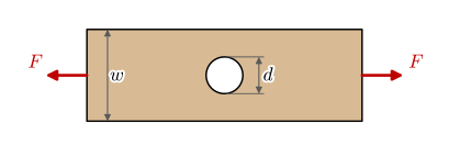
The nominal stress is part of the definition, and sources choose it differently. For a plate of width \(w\) and thickness \(t\) with a central hole of diameter \(d\), it can be taken on the net section through the hole, as in Example 4 of Chapter 8.4, or on the gross section away from it,

\[ \sigma_{\text{net}} = \frac{F}{(w - d)t}, \qquad \sigma_{\text{gross}} = \frac{F}{wt} . \]

Both describe the same peak, \(\sigma_{\max} = K_{t,\text{net}}\,\sigma_{\text{net}} = K_{t,\text{gross}}\,\sigma_{\text{gross}}\), so the two factors are related by

\[ K_{t,\text{gross}} = K_{t,\text{net}}\,\frac{\sigma_{\text{net}}}{\sigma_{\text{gross}}} = \frac{K_{t,\text{net}}}{1 - d/w} . \tag{8.15.2}\]

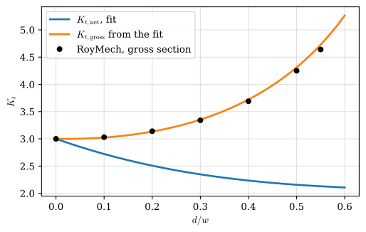
The net factor falls from \(3\) toward \(2\) as the hole grows, while the gross factor rises without bound, because the gross section keeps its area however little material is left beside the hole. RoyMech tabulates the gross factor¹, and Figure 8.15.1 compares that table with the net-section fit 8.4.3 converted by 8.15.2.

rho = np.linspace(0, 0.6, 200)                          # the hole diameter over the plate width, d/w
K_net = 3 - 3.140*rho + 3.667*rho**2 - 1.527*rho**3     # @eq-kt-hole, Pilkey (2005)
K_gross = K_net/(1 - rho)                               # @eq-kt-gross-net

# the same geometry tabulated on the gross section by RoyMech
rho_table = [0, 0.1, 0.2, 0.3, 0.4, 0.5, 0.55]
K_table = [3.00, 3.03, 3.14, 3.34, 3.69, 4.25, 4.64]

fig, ax = plt.subplots(figsize=(6, 3.6))
ax.plot(rho, K_net, color='C0', lw=2, label=r'$K_{t,\mathrm{net}}$, fit')
ax.plot(rho, K_gross, color='C1', lw=2, label=r'$K_{t,\mathrm{gross}}$ from the fit')
ax.plot(rho_table, K_table, 'o', color='k', ms=5, label='RoyMech, gross section')
ax.set_xlabel('$d/w$')
ax.set_ylabel('$K_t$')
ax.grid(True, alpha=0.4)
ax.legend()
plt.show()

The converted curve passes within two percent of the tabulated points, so the two sources agree once they refer to the same nominal stress. Taking a factor from one convention and a nominal stress from the other is the most common error with these charts, and at \(d/w = 0.5\) it is wrong by a factor of two.

A hole in a wide plate

The chart values are solutions of the continuum problem of Chapter 8.7, and one of them is known in closed form. In 1898 Kirsch solved the plane stress problem of a circular hole of radius \(a\) in an infinite plate under the remote tension \(\sigma\) [1]. His solution uses a stress function that satisfies equilibrium and compatibility identically, a technique beyond the scope of this book, so we take the result and check it. Figure 8.15.2 sets up the coordinates, with \(x\) along the load and the origin at the centre of the hole.

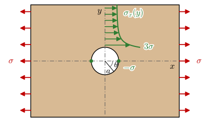
Along the cut \(x = 0\), the line through the centre of the hole perpendicular to the load, the stress in the load direction is

\[ \sigma_x(y) = \sigma\left(1 + \frac{a^2}{2y^2} + \frac{3a^4}{2y^4}\right), \qquad y \ge a . \tag{8.15.3}\]

At the edge of the hole, \(y = a\), the bracket is \(3\), the value quoted in Chapter 8.4, and far away it returns to \(1\). A sharper check is equilibrium. Cut the plate along the line \(x = 0\). The force across the cut is the same with and without the hole, so on each side of the hole the excess stress carried by the ligament must equal the force \(\sigma a\) (per unit thickness) that the missing material between \(y = 0\) and \(y = a\) would have carried,

\[ \int_a^\infty \left(\sigma_x - \sigma\right) dy = \sigma a . \]

y, a, sigma = sp.symbols('y a sigma', positive=True)
sigma_x = sigma*(1 + a**2/(2*y**2) + 3*a**4/(2*y**4))      # @eq-kirsch

ltx(r"\sigma_x(a) =", sigma_x.subs(y, a),
    r",\qquad \int_a^\infty (\sigma_x - \sigma)\,dy =", sp.integrate(sigma_x - sigma, (y, a, sp.oo)))

Both checks hold. Figure 8.15.3 shows how local the concentration is. One radius from the edge of the hole, at \(y = 2a\), the stress has fallen to \(1.22\sigma\), and at \(y = 3a\) the excess is below eight percent. The disturbance reaches about one hole diameter into the plate, as Saint-Venant’s principle of Section 8.3.9 leads us to expect, and it is why the width of a finite plate matters only when its edges come within that distance of the hole.

s = sp.lambdify(y, (sigma_x/sigma).subs(a, 1))              # sigma_x/sigma against y/a
ys = np.linspace(1, 5, 200)

fig, ax = plt.subplots(figsize=(6, 3.4))
ax.plot(ys, s(ys), color='C0', lw=2)
ax.fill_between(ys, 1, s(ys), color='C0', alpha=0.15, label=r'excess, area $\sigma a$')
ax.axhline(1, color='0.35', lw=0.8, ls='--')
for yk in (1, 2, 3):
    ax.plot(yk, s(yk), 'o', color='C3', ms=5)
    ax.annotate(f'{s(yk):.2f}', (yk, s(yk)), xytext=(8, 4), textcoords='offset points')
ax.set_xlabel('$y/a$')
ax.set_ylabel(r'$\sigma_x/\sigma$')
ax.set_ylim(0, 3.3)
ax.grid(True, alpha=0.4)
ax.legend()
plt.show()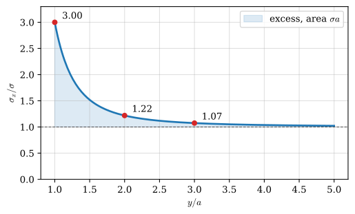

Around the rim of the hole the only stress is the hoop stress, \(\sigma_\theta = \sigma(1 - 2\cos 2\theta)\) with \(\theta\) measured from the load direction. It is \(3\sigma\) at \(\theta = \pm\pi/2\), where the cut \(x = 0\) meets the rim, and \(-\sigma\) at \(\theta = 0\) and \(\pi\), where the load axis meets it, Figure 8.15.2, so a plate in pure tension has a compressive stress at the rim of its hole. A brittle plate in compression cracks there, along the load.

Sharp notches

A circular hole is a mild discontinuity. In 1913 Inglis extended Kirsch’s solution to an elliptical hole with semi-axis \(a\) across the load and \(b\) along it [2]. The peak at the ends of the axis \(a\) is

\[ \sigma_{\max} = \sigma\left(1 + \frac{2a}{b}\right) = \sigma\left(1 + 2\sqrt{\frac{a}{\rho}}\right) \tag{8.15.4}\]

where \(\rho = b^2/a\) is the radius of curvature at the tip. A circle, \(a = b\), gives \(K_t = 3\) again. As the ellipse flattens into a crack, \(\rho \to 0\) and the peak grows without bound, so a sharp crack cannot be assessed with a stress concentration factor at all; that is the subject of fracture mechanics. For a finite tip radius, 8.15.4 says that the peak depends on the depth of the discontinuity relative to the radius at its root. A shallow scratch with a sharp root concentrates the stress more than a deep groove with a generous one.

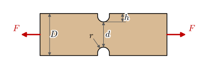
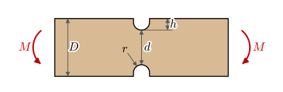
The same parameter governs a notch cut into the edge of a part, with the depth \(h\) in place of \(a\) and the root radius \(r\) in place of \(\rho\). For a groove in a shaft under torsion, where the shear stress flows around the root, the counterpart of 8.15.4 is \(1 + \sqrt{h/r}\), with half the square-root term. Both limits reappear in the handbook fits below.

Nominal stresses for the standard geometries

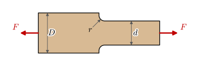
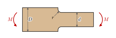
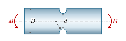
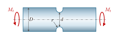
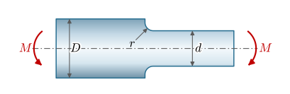
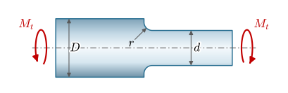
The geometries of this chapter are drawn in Figure 8.15.5 to Figure 8.15.13. A flat bar has the thickness \(t\), and a notch or a shoulder reduces its width from \(D\) to \(d\), removing the depth \(h = (D - d)/2\) on each side. A shaft has the diameters \(D\) and \(d\) in the same way. The nominal stress always refers to the smallest cross section, the net section through a hole and the section of width or diameter \(d\) at a notch, a groove or a shoulder.

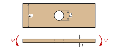
In tension the nominal stress is the force over the net area. In bending it is \(M/W\) with the section modulus \(W = I/c\) of 8.14.9. A rectangle \(d\) wide in the plane of bending and \(t\) thick has \(I = td^3/12\) and \(c = d/2\), so \(W = td^2/6\). Bending a plate with a hole out of its plane turns the net section on its side: it is \(w - d\) wide and \(t\) deep, and \(W = (w - d)t^2/6\). For a round section \(W = \pi d^3/32\) in bending and \(W = \pi d^3/16\) in torsion, by 8.11.5. Collected,

\[ \begin{aligned} &\text{hole:} && \sigma_{\text{nom}} = \frac{F}{(w - d)t}, && \sigma_{\text{nom}} = \frac{6M}{(w - d)t^2} \\ &\text{notch, shoulder:} && \sigma_{\text{nom}} = \frac{F}{dt}, && \sigma_{\text{nom}} = \frac{6M}{td^2} \\ &\text{shaft:} && \sigma_{\text{nom}} = \frac{32M}{\pi d^3}, && \tau_{\text{nom}} = \frac{16M_t}{\pi d^3} \end{aligned} \tag{8.15.5}\]

and the peak is \(K_t\) or \(K_{ts}\) times the matching nominal stress.

Curve fits to the charts

The charts were measured through the twentieth century with photoelastic models and strain gauges, and later recomputed with finite elements. Peterson’s collection is the standard reference [3]. For computation the curves have been fitted with polynomials [4,5], and for notches, grooves and shoulders all fits share one form,

\[ K_t = C_1 + C_2\left(\frac{2h}{D}\right) + C_3\left(\frac{2h}{D}\right)^2 + C_4\left(\frac{2h}{D}\right)^3, \qquad C_i = c_{i1} + c_{i2}\sqrt{h/r} + c_{i3}\,\frac{h}{r} \tag{8.15.6}\]

in which \(2h/D = 1 - d/D\) measures how much of the section the discontinuity removes. The coefficients \(c_{ij}\) come in two sets, one for \(h/r\) below \(2\) and one above, and each set holds only over the range of the data behind it. The square root is the parameter of 8.15.4. As \(2h/D \to 0\) the notch becomes shallow compared with the part and \(K_t \to C_1\), a function of \(h/r\) alone.

The plate with a hole has fits of its own. In tension it is 8.4.3. In bending out of its plane the factor depends also on the ratio of the hole diameter to the thickness [5],

\[ K_t = C\left[1 - 1.04\,\frac{d}{w} + 1.22\left(\frac{d}{w}\right)^2\right], \qquad C = 1.79 + \frac{0.25}{0.39 + d/t} + \frac{0.81}{1 + (d/t)^2} - \frac{0.26}{1 + (d/t)^3} \tag{8.15.7}\]

for \(d/w \le 0.3\). A thick plate, \(d/t \to 0\), gives \(C \to 2.98\): each layer of it is a plate in tension or compression with the factor \(3\) of 8.15.3. A thin plate, \(d/t \to \infty\), gives \(C \to 1.79\), the value of thin-plate bending theory.

The coefficients below are those of the references, with their ranges of validity. The function returns nan outside them, so that a chart or a calculation cannot quietly extrapolate a fit.

# The coefficients c_ij of @eq-kt-fit, one row (c_i1, c_i2, c_i3) per C_i, for h/r up to the
# switch and above it. Flat bars from Young (2012), round shafts from Pilkey (2005).
FITS = {
    'notch tension': dict(hr=(0.1, 2.0, 50.0),
        low=[(0.955, 2.169, -0.081), (-1.557, -4.046, 1.032), (4.013, 0.424, -0.748), (-2.461, 1.538, -0.236)],
        high=[(1.037, 1.991, 0.002), (-1.886, -2.181, -0.048), (0.649, 1.086, 0.142), (1.218, -0.922, -0.086)]),
    'notch bending': dict(hr=(0.1, 2.0, 50.0),
        low=[(1.024, 2.092, -0.051), (-0.630, -7.194, 1.288), (2.117, 8.574, -2.160), (-1.420, -3.494, 0.932)],
        high=[(1.113, 1.957, 0.0), (-2.579, -4.017, -0.013), (4.100, 3.922, 0.083), (-1.528, -1.893, -0.066)]),
    'step tension': dict(hr=(0.1, 2.0, 20.0),
        low=[(1.007, 1.000, -0.031), (-0.114, -0.585, 0.314), (0.241, -0.992, -0.271), (-0.134, 0.577, -0.012)],
        high=[(1.042, 0.982, -0.036), (-0.074, -0.156, -0.010), (-3.418, 1.220, -0.005), (3.450, -2.046, 0.051)]),
    'step bending': dict(hr=(0.1, 2.0, 20.0),
        low=[(1.007, 1.000, -0.031), (-0.270, -2.404, 0.749), (0.677, 1.133, -0.904), (-0.414, 0.271, 0.186)],
        high=[(1.042, 0.982, -0.036), (-3.599, 1.619, -0.431), (6.084, -5.607, 1.158), (-2.527, 3.006, -0.691)]),
    'groove bending': dict(hr=(0.25, 2.0, 50.0),
        low=[(0.594, 2.958, -0.520), (0.422, -10.545, 2.692), (0.501, 14.375, -4.486), (-0.613, -6.573, 2.177)],
        high=[(0.965, 1.926, 0.0), (-2.773, -4.414, -0.017), (4.785, 4.681, 0.096), (-1.995, -2.241, -0.074)]),
    'groove torsion': dict(hr=(0.25, 2.0, 50.0),
        low=[(0.966, 1.056, -0.022), (-0.192, -4.037, 0.674), (0.808, 5.321, -1.231), (-0.567, -2.364, 0.566)],
        high=[(1.089, 0.924, 0.018), (-1.504, -2.141, -0.047), (2.486, 2.289, 0.091), (-1.056, -1.104, -0.059)]),
    'shoulder bending': dict(hr=(0.1, 2.0, 20.0),
        low=[(0.947, 1.206, -0.131), (0.022, -3.405, 0.915), (0.869, 1.777, -0.555), (-0.810, 0.422, -0.260)],
        high=[(1.232, 0.832, -0.008), (-3.813, 0.968, -0.260), (7.423, -4.868, 0.869), (-3.839, 3.070, -0.600)]),
    'shoulder torsion': dict(hr=(0.25, 4.0, 4.0),       # a single set over the whole range
        low=[(0.905, 0.783, -0.075), (-0.437, -1.969, 0.553), (1.557, 1.073, -0.578), (-1.061, 0.171, 0.086)],
        high=[(0.905, 0.783, -0.075), (-0.437, -1.969, 0.553), (1.557, 1.073, -0.578), (-1.061, 0.171, 0.086)]),
}


def C_i(rows, q):
    """The four coefficients C_i of @eq-kt-fit at h/r = q."""
    return [c1 + c2*np.sqrt(q) + c3*q for c1, c2, c3 in rows]


def K_hole_bending(d_w, d_t):
    """@eq-kt-hole-bending at d/w = d_w and d/t = d_t, for a plate bent out of its plane."""
    C = 1.79 + 0.25/(0.39 + d_t) + 0.81/(1 + d_t**2) - 0.26/(1 + d_t**3)
    return np.where(d_w <= 0.3, C*(1 - 1.04*d_w + 1.22*d_w**2), np.nan)

Evaluating 8.15.6 is then a matter of computing \(h/r\) and \(2h/D\), picking the coefficient set, and summing the cubic.

def K_t(case, D, d, r):
    """The stress concentration factor of @eq-kt-fit, nan outside the fitted range."""
    lo, switch, hi = FITS[case]['hr']
    h = (D - d)/2
    q = np.asarray(h/r, dtype=float)
    x = 2*h/D
    C_low, C_high = C_i(FITS[case]['low'], q), C_i(FITS[case]['high'], q)
    K = sum(np.where(q <= switch, C_low[i], C_high[i])*x**i for i in range(4))
    return np.where((q >= lo) & (q <= hi), K, np.nan)

Figure 8.15.4 checks the shallow-notch limit \(C_1\) of three of the fits against the two Inglis limits. The fits were made to measured and computed charts with no reference to the elliptical hole, and they follow it closely over two decades of \(h/r\).

q = np.logspace(-1, np.log10(50), 200)                  # h/r


def C_1(case):
    lo, switch, hi = FITS[case]['hr']
    C = np.where(q <= switch, C_i(FITS[case]['low'], q)[0], C_i(FITS[case]['high'], q)[0])
    return np.where((q >= lo) & (q <= hi), C, np.nan)


fig, ax = plt.subplots(figsize=(6, 3.8))
ax.plot(q, 1 + 2*np.sqrt(q), color='k', lw=1, ls='--', label=r'Inglis, $1 + 2\sqrt{h/r}$')
ax.plot(q, 1 + np.sqrt(q), color='k', lw=1, ls=':', label=r'Inglis in shear, $1 + \sqrt{h/r}$')
ax.plot(q, C_1('notch tension'), color='C0', lw=2, label='notched bar, tension')
ax.plot(q, C_1('groove bending'), color='C1', lw=2, label='grooved shaft, bending')
ax.plot(q, C_1('groove torsion'), color='C2', lw=2, label='grooved shaft, torsion')
ax.set_xscale('log')
ax.set_xlabel('$h/r$')
ax.set_ylabel('$C_1$')
ax.grid(True, which='both', alpha=0.3)
ax.legend()
plt.show()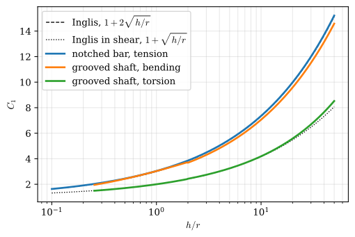

The standard cases

The charts below evaluate 8.15.6 for the five geometries of Figure 8.15.5 to Figure 8.15.13. Each curve is drawn only where its fit is valid, and where RoyMech tabulates the same geometry, its values are added as dots in the colour of the curve. They come from older handbook charts and scatter by several percent about the fits, which is the accuracy to expect from any of these sources.

Flat bar with a central hole

Code

rho = np.linspace(0, 0.8, 200)                          # d/w
fig, (ax1, ax2) = plt.subplots(1, 2, figsize=(9, 3.6), sharey=True)
ax1.plot(rho, 3 - 3.140*rho + 3.667*rho**2 - 1.527*rho**3, color='C0', lw=2)
ax1.set_title('tension')
for k, dt in enumerate([0.25, 0.5, 1, 2, 5]):
    ax2.plot(rho, K_hole_bending(rho, dt), color=f'C{k}', lw=2, label=f'$d/t = {dt}$')
ax2.set_title('bending out of the plane')
ax2.legend()
for ax in (ax1, ax2):
    ax.set_xlabel('$d/w$')
    ax.grid(True, alpha=0.4)
ax1.set_ylabel('$K_t$')
plt.show()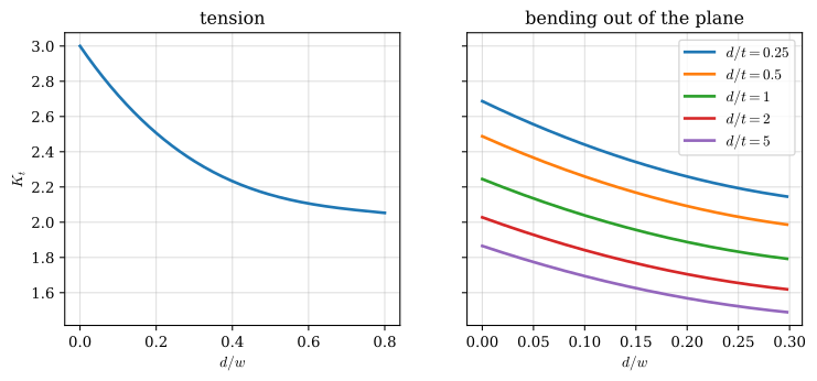

Flat bar with two U-notches

Code

# RoyMech's tables, {D/d: (r/d values, K_t values)}, for the geometries it covers
ROYMECH = {
    'step tension': {1.1: ([0.01, 0.02, 0.04, 0.06, 0.10, 0.15, 0.20, 0.25, 0.30],
                           [3.02, 2.43, 1.98, 1.78, 1.63, 1.51, 1.44, 1.39, 1.36]),
                     1.2: ([0.01, 0.02, 0.04, 0.06, 0.10, 0.15, 0.20, 0.25, 0.30],
                           [3.74, 2.98, 2.38, 2.14, 1.89, 1.72, 1.62, 1.56, 1.53]),
                     1.5: ([0.01, 0.02, 0.04, 0.06, 0.10, 0.15, 0.20, 0.25, 0.30],
                           [4.80, 3.75, 3.00, 2.64, 2.24, 1.99, 1.84, 1.74, 1.67])},
    'step bending': {1.1: ([0.01, 0.02, 0.04, 0.06, 0.10, 0.15, 0.20, 0.30],
                           [3.09, 2.45, 2.00, 1.80, 1.59, 1.49, 1.40, 1.31]),
                     1.2: ([0.01, 0.02, 0.04, 0.06, 0.10, 0.15, 0.20, 0.30],
                           [3.62, 2.81, 2.23, 1.97, 1.70, 1.55, 1.44, 1.34]),
                     1.5: ([0.01, 0.02, 0.04, 0.06, 0.10, 0.15, 0.20, 0.30],
                           [3.80, 2.98, 2.38, 2.15, 1.83, 1.63, 1.52, 1.38]),
                     2.0: ([0.02, 0.04, 0.06, 0.10, 0.15, 0.20, 0.30],
                           [3.14, 2.59, 2.23, 1.88, 1.66, 1.54, 1.40])},
    'groove bending': {1.1: ([0.04, 0.06, 0.10, 0.15, 0.20, 0.25, 0.30],
                             [2.45, 2.14, 1.85, 1.64, 1.53, 1.45, 1.39]),
                       1.2: ([0.04, 0.06, 0.10, 0.15, 0.20, 0.25, 0.30],
                             [2.63, 2.30, 1.92, 1.70, 1.57, 1.48, 1.42]),
                       1.5: ([0.04, 0.06, 0.10, 0.15, 0.20, 0.25, 0.30],
                             [2.85, 2.40, 2.00, 1.74, 1.60, 1.51, 1.43]),
                       2.0: ([0.04, 0.06, 0.10, 0.15, 0.20, 0.25, 0.30],
                             [2.95, 2.45, 2.10, 1.83, 1.67, 1.55, 1.45])},
    'groove torsion': {1.1: ([0.02, 0.03, 0.04, 0.06, 0.10, 0.15, 0.20, 0.30],
                             [2.00, 1.84, 1.74, 1.63, 1.45, 1.35, 1.29, 1.22]),
                       1.2: ([0.02, 0.03, 0.04, 0.06, 0.10, 0.15, 0.20, 0.30],
                             [2.16, 1.97, 1.85, 1.69, 1.51, 1.39, 1.32, 1.24]),
                       1.5: ([0.02, 0.03, 0.04, 0.06, 0.10, 0.15, 0.20, 0.30],
                             [2.24, 2.03, 1.90, 1.73, 1.53, 1.39, 1.30, 1.25])},
    'shoulder bending': {1.2: ([0.01, 0.02, 0.03, 0.04, 0.05, 0.08, 0.10, 0.15, 0.20, 0.25],
                               [3.30, 2.60, 2.30, 2.10, 1.95, 1.75, 1.65, 1.50, 1.42, 1.30]),
                         1.5: ([0.01, 0.02, 0.03, 0.04, 0.05, 0.08, 0.10, 0.15, 0.20, 0.25],
                               [3.73, 2.90, 2.52, 2.30, 2.13, 1.84, 1.72, 1.54, 1.43, 1.35]),
                         2.0: ([0.01, 0.02, 0.03, 0.04, 0.05, 0.08, 0.10, 0.15, 0.20, 0.25],
                               [3.70, 3.17, 2.71, 2.42, 2.25, 1.92, 1.78, 1.58, 1.46, 1.36])},
    'shoulder torsion': {1.1: ([0.02, 0.03, 0.05, 0.07, 0.10, 0.15, 0.20, 0.30],
                               [1.72, 1.57, 1.43, 1.35, 1.28, 1.21, 1.17, 1.12]),
                         1.2: ([0.02, 0.03, 0.05, 0.07, 0.10, 0.15, 0.20, 0.30],
                               [2.00, 1.70, 1.57, 1.42, 1.33, 1.25, 1.20, 1.15]),
                         1.5: ([0.02, 0.03, 0.05, 0.07, 0.10, 0.15, 0.20, 0.30],
                               [2.20, 1.92, 1.62, 1.47, 1.36, 1.25, 1.20, 1.14]),
                         2.0: ([0.02, 0.03, 0.05, 0.07, 0.10, 0.15, 0.20, 0.30],
                               [2.55, 2.15, 1.75, 1.60, 1.45, 1.31, 1.24, 1.16])},
}


def chart(cases, titles, ratios=(1.1, 1.2, 1.5, 2.0), ylabel='$K_t$'):
    """K_t of @eq-kt-fit against r/d for several D/d, one panel per load case."""
    rd = np.linspace(0.01, 0.3, 300)
    fig, axes = plt.subplots(1, len(cases), figsize=(9, 3.6), sharey=True)
    for ax, case, title in zip(axes, cases, titles):
        for k, Dd in enumerate(ratios):
            ax.plot(rd, K_t(case, Dd, 1.0, rd), color=f'C{k}', lw=2, label=f'$D/d = {Dd}$')
            if Dd in ROYMECH.get(case, {}):
                ax.plot(*ROYMECH[case][Dd], 'o', color=f'C{k}', ms=4)
        ax.set_title(title)
        ax.set_xlabel('$r/d$')
        ax.set_ylim(1, 4)
        ax.grid(True, alpha=0.4)
    axes[0].set_ylabel(ylabel)
    axes[-1].legend()
    plt.show()

Code

chart(['notch tension', 'notch bending'], ['tension', 'bending'], ratios=(1.1, 1.2, 1.5, 2.0, 3.0))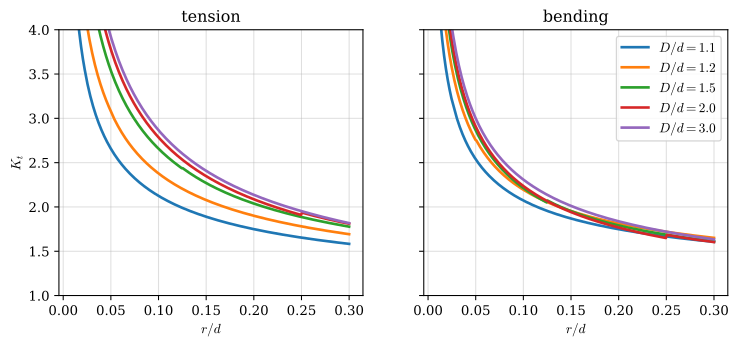

Stepped flat bar

Code

chart(['step tension', 'step bending'], ['tension', 'bending'])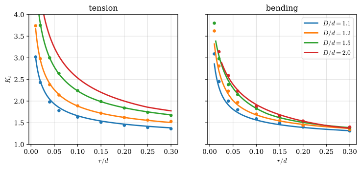

Round shaft with a U-groove

Code

chart(['groove bending', 'groove torsion'], ['bending, $K_t$', 'torsion, $K_{ts}$'],
      ylabel='$K_t$, $K_{ts}$')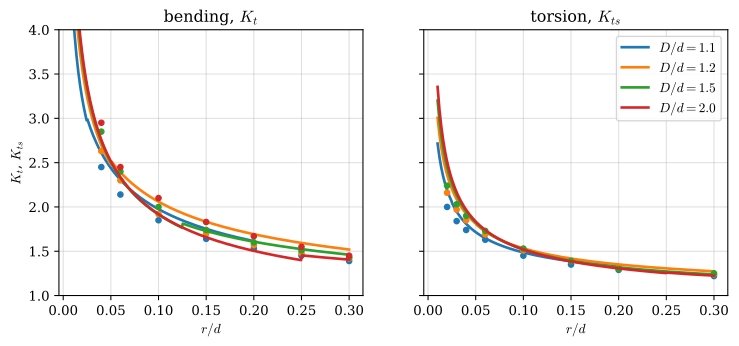

Stepped round shaft

Code

chart(['shoulder bending', 'shoulder torsion'], ['bending, $K_t$', 'torsion, $K_{ts}$'],
      ylabel='$K_t$, $K_{ts}$')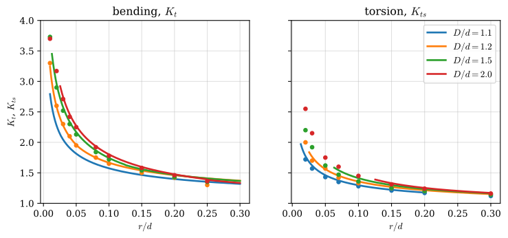

The charts share a pattern. Every factor falls as the radius grows, steeply at first and then slowly, as the square root in 8.15.6 predicts. A deeper discontinuity, a larger \(D/d\), raises the factor at first, but beyond \(D/d \approx 1.5\) hardly at all, because the far part of the wide section carries little of the load around the corner. For the grooved shaft the curves of the deeper grooves even cross, which is within the scatter of the data behind the fits. Torsion concentrates less than bending of the same shaft, and a shoulder less than a groove of the same depth.

Example 1: A shaft shoulder in bending and torsion

A steel shaft steps down from \(D = 40~\text{mm}\) to \(d = 32~\text{mm}\) at the shoulder of a bearing seat, with a fillet of radius \(r = 2~\text{mm}\) as in Figure 8.15.13. At the shoulder the shaft carries the bending moment \(M = 200~\text{N\,m}\) and the torque \(M_t = 300~\text{N\,m}\). The steel has the yield strength \(\sigma_y = 500~\text{MPa}\). Determine the peak stresses in the fillet and the factor of safety against yielding, and find how both depend on the fillet radius.

The shoulder has the height \(h = (D - d)/2 = 4~\text{mm}\), so \(h/r = 2\) and \(2h/D = 0.2\), inside the range of both fits. The nominal stresses of 8.15.5 and the peaks are

\[ \sigma_{\text{nom}} = \frac{32M}{\pi d^3}, \quad \sigma_{\max} = K_t\,\sigma_{\text{nom}}, \qquad \tau_{\text{nom}} = \frac{16M_t}{\pi d^3}, \quad \tau_{\max} = K_{ts}\,\tau_{\text{nom}} \]

with \(K_t\) and \(K_{ts}\) from 8.15.6. The bending peak lies at the top and the bottom of the section and the torsion peak all around it, so at the top of the fillet both act at once. The surface there is free of load, which leaves a plane stress state with \(\sigma_x = \sigma_{\max}\), \(\sigma_y = 0\) and \(\tau_{xy} = \tau_{\max}\), and 8.7.16 gives

\[ \sigma_{\text{vM}} = \sqrt{\sigma_{\max}^2 + 3\tau_{\max}^2}, \qquad \eta = \frac{\sigma_y}{\sigma_{\text{vM}}} . \]

The two peaks do not fall on exactly the same point of the fillet, so combining them is slightly conservative.

D, d, r = 40, 32, 2                  # mm
M, M_t = 200e3, 300e3                # N mm, so stresses in MPa
sigma_y = 500

sigma_nom = 32*M/(np.pi*d**3)
tau_nom = 16*M_t/(np.pi*d**3)
K_b = K_t('shoulder bending', D, d, r)
K_s = K_t('shoulder torsion', D, d, r)
sigma_max, tau_max = K_b*sigma_nom, K_s*tau_nom
sigma_vM = np.sqrt(sigma_max**2 + 3*tau_max**2)

ltx(r"\sigma_{\text{nom}} &=", sigma_nom, r"~\text{MPa}, \quad K_t =", K_b,
    r", \quad \sigma_{\max} =", sigma_max, r"~\text{MPa}",
    r"\\ \tau_{\text{nom}} &=", tau_nom, r"~\text{MPa}, \quad K_{ts} =", K_s,
    r", \quad \tau_{\max} =", tau_max, r"~\text{MPa}",
    r"\\ \sigma_{\text{vM}} &=", sigma_vM, r"~\text{MPa}, \quad \eta =", sigma_y/sigma_vM,
    aligned=True, precision=3)

Without the shoulder the von Mises stress would be \(\sqrt{\sigma_{\text{nom}}^2 + 3\tau_{\text{nom}}^2} = 102~\text{MPa}\), so the fillet raises it by two thirds. The factor of safety of about \(3\) looks comfortable for a static load, but a rotating shaft sees the bending stress reverse on every turn, and in fatigue the peak in the fillet is what counts. Figure 8.15.15 repeats the calculation for other fillet radii.

r_range = np.linspace(1, 8, 200)
vM = np.sqrt((K_t('shoulder bending', D, d, r_range)*sigma_nom)**2
             + 3*(K_t('shoulder torsion', D, d, r_range)*tau_nom)**2)

fig, ax = plt.subplots(figsize=(6, 3.6))
ax.plot(r_range, vM, color='C0', lw=2, label=r'$\sigma_{\mathrm{vM}}$ in the fillet')
ax.axhline(np.sqrt(sigma_nom**2 + 3*tau_nom**2), color='0.35', ls='--', lw=1,
           label='without the shoulder')
ax.plot(r, sigma_vM, 'o', color='C3', label=f'$r = {r}$ mm')
ax.set_xlabel('fillet radius $r$ [mm]')
ax.set_ylabel('stress [MPa]')
ax.set_ylim(0, 220)
ax.grid(True, alpha=0.4)
ax.legend()
plt.show()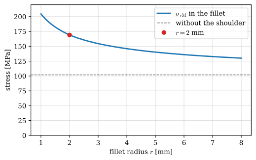

Halving the radius to \(1~\text{mm}\) raises the peak to \(205~\text{MPa}\), and doubling it to \(4~\text{mm}\) lowers it to \(146~\text{MPa}\). The designer is rarely free to choose, because the inner ring of the bearing has a corner radius of its own and must seat against the shoulder, so the fillet has to be smaller than that corner. Where a larger fillet will not fit, an undercut into the shoulder face or a spacer ring with a large bore chamfer allows a larger radius in the shaft.

Example 2: Three ways to narrow a bar

The steel plate of Example 4 in Chapter 8.4 is \(w = 40~\text{mm}\) wide and \(t = 5~\text{mm}\) thick, carries \(F = 20~\text{kN}\) and has a hole of \(d = 12~\text{mm}\), with \(\sigma_y = 355~\text{MPa}\). Suppose the same net width of \(28~\text{mm}\) were reached instead by two U-notches of depth \(h = 6~\text{mm}\) with root radius \(r = 3~\text{mm}\), Figure 8.15.7, or by stepping the bar down to \(d = 28~\text{mm}\) with fillets of \(r = 3~\text{mm}\), Figure 8.15.9. Compare the peak stresses of the three designs.

All three have the same smallest section, so by 8.15.5 they share one nominal stress,

\[ \sigma_{\text{nom}} = \frac{F}{(w - d)t} = \frac{F}{dt} = \frac{20\,000}{28 \cdot 5}~\text{MPa} = 143~\text{MPa} . \]

The hole has \(d/w = 0.3\) in 8.4.3. The notch and the step both have \(h/r = 2\) and \(2h/D = 0.3\) in 8.15.6, with their own coefficients. Each peak is \(\sigma_{\max} = K_t\sigma_{\text{nom}}\), and each factor of safety against local yielding is \(\eta = \sigma_y/\sigma_{\max}\).

F, w, t = 20e3, 40, 5                # N and mm
sigma_y = 355
sigma_nom = F/(28*t)

designs = {r"\text{hole}": 3 - 3.140*0.3 + 3.667*0.3**2 - 1.527*0.3**3,
           r"\text{notches}": K_t('notch tension', 40, 28, 3),
           r"\text{step}": K_t('step tension', 40, 28, 3)}

rows = []
for name, K in designs.items():
    rows += [("" if not rows else r"\\ ") + name + r": \quad K_t &=", K,
             r", \quad \sigma_{\max} =", K*sigma_nom, r"~\text{MPa}, \quad \eta =",
             sigma_y/(K*sigma_nom)]
ltx(*rows, aligned=True, precision=3)

The notches are worst, the step is best, and the hole lies between them, although the three designs remove the same material from the same section. The peaks differ by twenty percent. At the notch the lines of force turn in toward the waist and back out again within a length of \(2r\), while at the step they turn once and then run straight on. With the notches the peak even exceeds the yield strength, \(\eta < 1\). As discussed in Chapter 8.4, a ductile steel under a static load yields in a thin layer at the root and carries on, since the net section has \(\eta = 355/143 = 2.5\), but under a varying load that layer is where a fatigue crack starts. Figure 8.15.16 shows how the radius changes the ranking.

r_range = np.linspace(1, 10, 200)

fig, ax = plt.subplots(figsize=(6, 3.6))
ax.plot(r_range, K_t('notch tension', 40, 28, r_range), color='C0', lw=2, label='two U-notches')
ax.plot(r_range, K_t('step tension', 40, 28, r_range), color='C1', lw=2, label='step with fillets')
ax.axhline(designs[r"\text{hole}"], color='C2', lw=2, label='hole, $d = 12$ mm')
ax.axvline(3, color='0.35', lw=0.8, ls='--')
ax.set_xlabel('root or fillet radius $r$ [mm]')
ax.set_ylabel('$K_t$')
ax.grid(True, alpha=0.4)
ax.legend()
plt.show()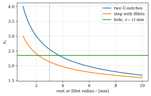

Larger radii help both alternatives. At \(r = 6~\text{mm}\), where the notch is a semicircle as deep as its radius, its factor falls to \(2.0\) and that of the step to \(1.8\), both below the hole.

Other geometries and the finite element method

The charts cover a finite list of shapes, and handbooks extend the list to keyways, cross holes, threads, splines and many more [3]. When no chart matches, or when a chart is not accurate enough, the stress concentration has to be computed, and a finite element model of the part with a fine mesh at the discontinuity gives the peak directly. The finite element notebook of Section 8.4.5 does this for the plate with a hole and reproduces 8.4.3. The same procedure applies to any shape, which brings us back to the continuum model of Chapter 8.7: every chart in this chapter is a tabulated solution of that model, and a computation replaces the table.

Stress concentration in design

Whether the peak matters depends on the material and on the load. A ductile metal under a static load yields in a thin layer where the stress is highest, the stress spreads over the rest of the section, and the part carries on. Its static strength is then set by the net section, and \(K_t\) plays almost no role. A brittle material cannot redistribute the stress, and it fails when the peak reaches its strength. Under a varying load every material behaves in the brittle way, because fatigue cracks start at the peak.

In fatigue a sharp notch in a ductile metal does less harm than \(K_t\) predicts, since the stress falls off so steeply from the root that only a very small volume of material sees the peak. Design codes account for this with the fatigue notch factor

\[ K_f = 1 + q\,(K_t - 1) \tag{8.15.8}\]

where the notch sensitivity \(q\) lies between \(0\), for a material that ignores the notch, and \(1\), for one that feels the full \(K_t\). It depends on the material and the root radius, approaching \(1\) for high-strength steels and large radii, and it is tabulated in machine design texts [6].

The remedies follow from 8.15.4. The largest radius the design allows is the most effective one, and since the factor grows with the square root of \(h/r\), a sharp internal corner with \(r\) close to zero is the most damaging feature a part can have. In a 3D-printed bracket, rounding such a corner off adds nothing to the print time. A discontinuity should sit where the nominal stress is low, away from the section of the largest moment. Removing more material can help as well. A hole drilled at the tip of a crack replaces a tip of radius close to zero with the radius of the hole, and relief grooves cut beside a sharp shoulder make the lines of force turn more gradually.

References

[1]
Kirsch EG. Die theorie der elastizität und die bedürfnisse der festigkeitslehre. Zeitschrift Des Vereines Deutscher Ingenieure 1898;42:797–807.
[2]
Inglis CE. Stresses in a plate due to the presence of cracks and sharp corners. Transactions of the Institution of Naval Architects 1913;55:219–41.
[3]
Pilkey WD, Pilkey DF. Peterson’s stress concentration factors. 3rd ed. Hoboken, NJ: John Wiley & Sons; 2008.
[4]
Pilkey WD. Formulas for stress, strain, and structural matrices. 2nd ed. Hoboken, NJ: John Wiley & Sons; 2005.
[5]
Young WC, Budynas RG, Sadegh AM. Roark’s formulas for stress and strain. 8th ed. New York: McGraw-Hill; 2012.
[6]
Budynas RG, Nisbett JK. Shigley’s mechanical engineering design. 11th ed. New York: McGraw-Hill Education; 2020.
RoyMech, Stress concentration factors: https://www.roymech.co.uk/Useful_Tables/Fatigue/Stress_concentration.html↩︎