The assumptions

Four assumptions define the Euler-Bernoulli beam, also known as the engineering beam theory. The deformations are assumed to be small, so that the linear strain measure 8.7.3 applies. The material is linearly elastic. Poisson effects are neglected, so that the axial stress follows the one-dimensional Hooke’s law \(\sigma = E\varepsilon\) rather than the full 8.9.7. Finally, and this is the assumption that does the work, every cross section remains plane and perpendicular to the neutral axis during deformation.

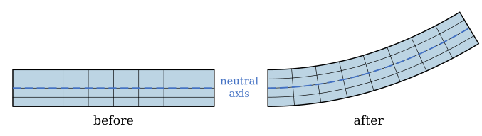
The last assumption is a statement about geometry, and it is what Figure 8.16.1 illustrates. Longitudinal lines in the beam become curved, while lines that were vertical stay straight and merely rotate. Somewhere between the top and the bottom is a surface that neither stretches nor shortens: the neutral plane, whose intersection with the plane of bending is the neutral axis. For a homogeneous beam the neutral axis passes through the centroid of the cross section, which is why the second moment of area is always taken about the centroid.

Although the Euler-Bernoully theory involves many assumptions and simplifications, it provides accurate prediction for many important practical engineering problems.

Kinematics

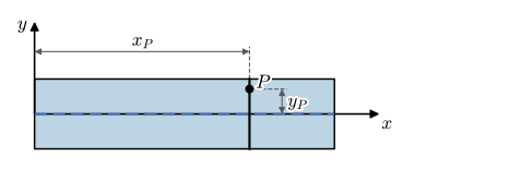
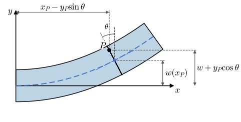
Let \(x\) run along the beam, \(y\) across it in the plane of bending and \(z\) out of that plane, with the \(x\) axis along the neutral axis of the undeformed beam. The deflection \(w(x)\) is the displacement of the neutral axis in the \(y\) direction, positive upward. Consider a material point \(P\) at \(\bm r_P = [x_P, y_P, z_P]^\mathsf{T}\) before deformation, as in Figure 8.16.2. Its cross section moves with the axis by \(w\) and turns through an angle \(\theta\).

Reading the dimensions off the after panel, the point has moved to

\[ \bm r_P' = \begin{bmatrix} x_P - y_P \sin\theta\\ w(x_P) + y_P \cos\theta\\ z_P \end{bmatrix} \tag{8.16.1}\]

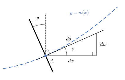
The rotation angle is not independent, and 8.16.1 already shows why. A point on the neutral axis has \(y_P = 0\), so it moves straight up by \(w\) and not sideways, and the deformed axis is the curve \(y = w(x)\), the graph of the deflection. Its slope is read off the graph as for any function. Seen closely enough the axis is straight, and over a short run \(dx\) it rises \(dw\) along the hypotenuse \(ds\) of the right triangle in Figure 8.16.3. The angle \(\theta\) between the axis and the horizontal lies opposite the rise and next to the run, so

\[ \tan\theta = \frac{dw}{dx} = w' \tag{8.16.2}\]

The cross section is held at right angles to that tangent. Two lines at a right angle turn together, like the two arms of a set square, so when the tangent has turned \(\theta\) from the horizontal the section has turned the same \(\theta\) from the vertical. This is the angle in 8.16.1.

The angles are small. A beam in service rarely deflects more than about \(1/300\) of its span, which for a simply supported beam under a uniform load gives a largest slope near \(w' = 0.01\). At that slope \(\tan\theta\) and \(\theta\) differ by \(\theta^3/3 \approx 3\cdot 10^{-7}\) and \(\cos\theta\) differs from 1 by \(\theta^2/2 = 5\cdot 10^{-5}\), so we may take \(\sin\theta \approx \theta \approx \tan\theta = w'\) and \(\cos\theta \approx 1\). The displacement of \(P\) becomes

\[ \bm u = \bm r_P' - \bm r_P = \begin{bmatrix} -y_P\,\theta\\ w\\ 0 \end{bmatrix} \]

Since \(P\) was any point of the beam, we drop the subscript and obtain the displacement field

\[ \bm u(x, y, z) = \begin{bmatrix} -y\, \dfrac{dw}{dx}\\[8pt] w\\ 0 \end{bmatrix} \tag{8.16.3}\]

A three-dimensional vector field has been reduced to one scalar function \(w(x)\) of one variable. Everything else in this chapter is bookkeeping applied to 8.16.3.

Curvature

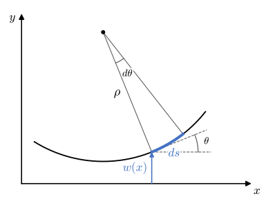
How sharply the beam bends is measured by the curvature of its axis. An element \(ds\) of the deflected axis lies on a circle of radius \(\rho\) about the centre of curvature, Figure 8.16.4, and seen from that centre it spans the angle \(d\theta\), so that \(ds = \rho\,d\theta\).

The curvature is the rate at which the slope angle turns along the axis,

\[ \kappa = \frac{1}{\rho} = \frac{d\theta}{ds} \]

and for small slopes \(ds \approx dx\) and \(\theta \approx w'\), so that

\[ \boxed{\kappa = \frac{1}{\rho} = \frac{d^2 w}{dx^2}} \tag{8.16.4}\]

This is the small-slope limit of the exact curvature of a plane curve, \(\kappa = w''/(1 + w'^2)^{3/2}\). The curvature is positive when the axis bends upward, with the centre of curvature above it as in the figure.

Strain and stress

The strain is the symmetric part of the displacement gradient, 8.7.3,

\[ \bm\varepsilon = \tfrac12\left(\nabla\bm u + \nabla\bm u^\mathsf{T}\right) \]

applied to 8.16.3. We let SymPy form both instead of differentiating nine entries by hand.

x, y, z = sp.symbols('x y z', real=True)
E_mod = sp.symbols('E', positive=True)

w = sp.Function('w')(x)

uu = sp.Matrix([-y*sp.diff(w, x), w, 0])
XX = sp.Matrix([x, y, z])

grad_u = uu.jacobian(XX)
eps = sp.simplify((grad_u + grad_u.T)/2)

ltx(r"\nabla \bm u =", grad_u, r",\qquad \bm\varepsilon = \tfrac12(\nabla\bm u + \nabla\bm u^\mathsf{T}) =", eps)

The displacement gradient has two non-zero entries, but its symmetric part has only one. The off-diagonal terms \(-w'\) and \(+w'\) cancel exactly, which is the algebraic signature of the perpendicularity assumption: the cross section rotates rigidly with the axis, and a rigid rotation produces no strain. What survives is a single axial strain, which with 8.16.4 reads

\[ \boxed{\varepsilon_{xx} = -y \frac{d^2 w}{dx^2} = -\frac{y}{\rho}} \tag{8.16.5}\]

proportional to the distance from the neutral axis and to the curvature of the beam. Fibres above the neutral axis (\(y > 0\)) shorten when the curvature is positive, fibres below it stretch, and the fibre on the axis does neither, which is what earned it the name.

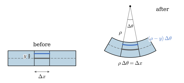
The geometry of the bent beam gives the same strain without the displacement gradient, which makes a check on the continuum route. In Figure 8.16.5 a piece \(\Delta x\) of the beam bends into an arc that spans the angle \(\Delta\theta\) about the centre of curvature. The neutral axis keeps its length, \(\rho\,\Delta\theta = \Delta x\). A fibre at the height \(y\) lies nearer the centre, on the radius \(\rho - y\), so its length becomes \((\rho - y)\,\Delta\theta\) and its strain is

\[ \varepsilon_{xx} = \frac{(\rho - y)\,\Delta\theta - \rho\,\Delta\theta}{\rho\,\Delta\theta} = -\frac{y}{\rho} \]

The difference between the fibre strain and the entry \(\varepsilon_{xx}\) of the displacement gradient, with \(w'' = 1/\rho\), should vanish.

rho, dtheta = sp.symbols(r'rho \Delta\theta', positive=True)

eps_fibre = ((rho - y)*dtheta - rho*dtheta)/(rho*dtheta)     # the fibre of the figure
eps_continuum = eps[0, 0].subs(sp.diff(w, x, 2), 1/rho)       # from the displacement gradient

ltx(r"\varepsilon_{\text{fibre}} - \varepsilon_{xx} =", sp.simplify(eps_fibre - eps_continuum))

The two routes agree. The stress follows from Hooke’s law, and since we have neglected Poisson effects it is the one-dimensional form,

\[ \bm\sigma = E\bm\varepsilon \]

sigma = sp.simplify(E_mod*eps)
ltx(r"\bm\sigma = E\bm\varepsilon =", sigma)

so that the only non-zero stress component is

\[ \boxed{\sigma_{xx} = -E y \frac{d^2 w}{dx^2}} \tag{8.16.6}\]

The stress varies linearly through the depth of the section, from maximum compression at one surface through zero at the neutral axis to maximum tension at the other. Material near the neutral axis is barely worked at all, which is why I-beams and box sections put their material at the extremes and why a hollow tube is so much more efficient in bending than a solid rod of the same mass.

nu = sp.symbols('nu', positive=True)
mu_lame = E_mod/(2*(1 + nu))                          # @eq-lame
lam_lame = E_mod*nu/((1 + nu)*(1 - 2*nu))

# the generalized Hooke's law applied to the strain of the beam
sigma_full = sp.simplify(2*mu_lame*eps + lam_lame*eps.trace()*sp.eye(3))
ltx(r"\bm\sigma = 2\mu\bm\varepsilon + \lambda\operatorname{tr}(\bm\varepsilon)\bm I =", sigma_full)

Internal forces and the second moment of area

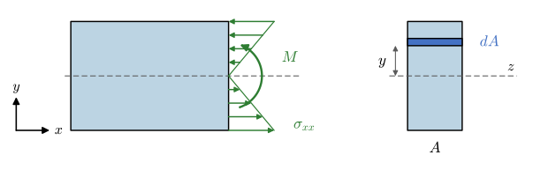
The stress distribution 8.16.6 must be statically equivalent to the internal forces on the cut, Figure 8.16.6. A strip \(dA = dy\,dz\) at the height \(y\) carries the force \(\sigma_{xx}\,dA\) at the lever arm \(y\) from the neutral axis.

We take the moment on a face with outward normal \(+x\) as positive anticlockwise, the sense of Figure 8.16.6. Its resultant about the \(z\) axis is the stress times its lever arm integrated over the cross section,

\[ \begin{aligned} M &= \iint -y\,\sigma_{xx}\,dy\,dz = \iint E y^2 \frac{d^2 w}{dx^2}\,dy\,dz \\ &= E\frac{d^2 w}{dx^2} \underbrace{\iint y^2\,dy\,dz}_{I} \end{aligned} \]

where the curvature came out of the integral because it does not vary over the cross section. The remaining integral is a purely geometric property,

\[ \boxed{I = \iint y^2\, dy\, dz} \tag{8.16.8}\]

the second moment of area about the neutral axis, with units of length to the fourth power. This gives the moment-curvature relation

\[ \boxed{M = EI \frac{d^2 w}{dx^2} = \frac{EI}{\rho}} \tag{8.16.9}\]

in which the product \(EI\) appears as a single quantity, the bending stiffness. Material and geometry enter only through their product, so a stiffer material and a deeper section are interchangeable as far as deflection is concerned.

Eliminating the curvature between 8.16.6 and 8.16.9 gives the result that every engineer knows,

\[ \boxed{\sigma_{xx} = -\frac{M y}{I}} \tag{8.16.10}\]

and evaluating it at the extreme fibre, at distance \(c\) from the neutral axis, gives the maximum bending stress

\[ \sigma_{\max} = \frac{Mc}{I} = \frac{M}{W}, \qquad W := \frac{I}{c} \tag{8.16.11}\]

where \(W\) is the section modulus, the single number that determines how much moment a section can carry at a given stress. Values of \(I\) and \(W\) for standard sections are tabulated in every handbook, and a CAD system reports them for arbitrary sections directly. For a rectangle of width \(b\) and height \(h\) the integral is elementary.

b, h_sec = sp.symbols('b h', positive=True)

I_rect = sp.integrate(sp.integrate(y**2, (y, -h_sec/2, h_sec/2)), (z, 0, b))
W_rect = sp.simplify(I_rect/(h_sec/2))

ltx(r"I_{\text{rect}} &=", I_rect, r"\\ W_{\text{rect}} &=", W_rect, aligned=True)

The height enters \(I\) cubed. Doubling the height of a beam makes it eight times stiffer and four times stronger, while doubling its width does neither more than doubling. This single fact governs almost every decision about how to orient a structural member.

Equilibrium of a slice

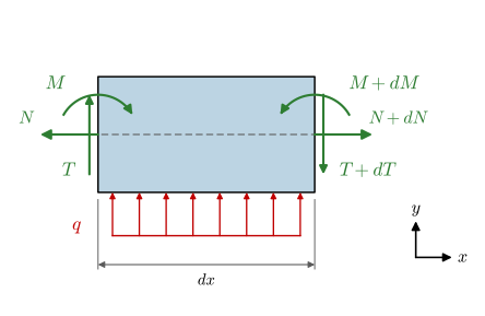
8.16.9 relates the moment to the deflection, but nothing yet relates the moment to the applied load. That link comes from equilibrium, applied not to the whole beam but to a slice of length \(dx\) carrying a distributed load \(q\) per unit length, Figure 8.16.7. The internal forces on the left face of the slice are a normal force \(N\), a shear force \(T\) and a bending moment \(M\), and on the right face each has changed by its own derivative times \(dx\).

Vertical force equilibrium of the slice and moment equilibrium about the centre of its right face, with anticlockwise moments positive, read

\[ \begin{aligned} T - (T + dT) + q\,dx &= 0 \\ -M + (M + dM) - T\,dx - q\,dx\,\frac{dx}{2} &= 0 \end{aligned} \]

and dropping the term of second order in \(dx\) leaves the change in shear force as the applied load and the change in bending moment as the shear force,

\[ \frac{dT}{dx} = q, \qquad \frac{dM}{dx} = T \tag{8.16.12}\]

These two relations are worth committing to memory in their own right, because they say that the shear diagram is the integral of the load and the moment diagram is the integral of the shear. A moment diagram has a maximum wherever the shear crosses zero, and the shear jumps by exactly the size of any point load.

Two standard cases show both rules. A cantilever with a point load at the free end carries no distributed load, so \(T\) is constant and \(M\) is linear in \(x\): zero at the free end and largest at the clamped end, where a downward tip force \(P\) gives \(M = -PL\). A simply supported beam with a uniformly distributed load has \(T\) linear in \(x\) and zero at midspan, so the moment peaks there, and a downward load of magnitude \(q_0\) gives \(M_{\max} = q_0L^2/8\) while \(M\) vanishes at both supports.

The elastic line equation

Now assemble the pieces. Substituting the moment-curvature relation 8.16.9 into 8.16.12 twice gives

\[ \boxed{EI \frac{d^4 w}{dx^4} = q(x)} \tag{8.16.13}\]

the elastic line equation, a fourth-order ordinary differential equation for the deflection. The three-dimensional continuum problem has been reduced to this. Everything that made the general problem hard, the coupling between displacement components and the two extra spatial dimensions, was eliminated by the kinematic assumption.

Because 8.16.13 is obtained by differentiating 8.16.9, the intermediate derivatives are all quantities we have names for. Integrating downward from the load gives a ladder,

\[ \begin{array}{llll} EI\,\dfrac{d^4w}{dx^4} = q(x) & \quad\text{load} \\[8pt] EI\,\dfrac{d^3w}{dx^3} = T(x) & \quad\text{shear force} \\[8pt] EI\,\dfrac{d^2w}{dx^2} = M(x) & \quad\text{bending moment} \\[8pt] \dfrac{dw}{dx} = \theta(x) & \quad\text{slope} \\[8pt] w(x) & \quad\text{deflection} \end{array} \tag{8.16.14}\]

so a single solution of 8.16.13 produces the shear diagram, the moment diagram, the rotation and the deflection at once, together with the bending stress through 8.16.10. There is no need to draw shear and moment diagrams by hand as a separate exercise: they are derivatives of the answer.

Boundary conditions

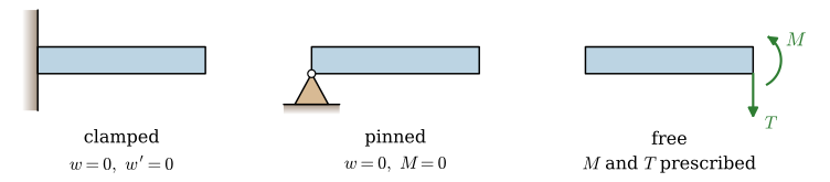
A fourth-order equation needs four conditions, two at each end. At each end there are four quantities available, and exactly two of them may be prescribed: the deflection, the slope, the moment and the shear force. Which two depends on the support.

\[ \begin{array}{ll} w(0) = 0 & \qquad w(L) = 0\\[4pt] \dfrac{dw}{dx}(0) = 0 & \qquad \dfrac{dw}{dx}(L) = 0\\[8pt] \dfrac{d^2w}{dx^2}(0) = \dfrac{M}{EI} & \qquad \dfrac{d^2w}{dx^2}(L) = \dfrac{M}{EI}\\[8pt] \dfrac{d^3w}{dx^3}(0) = \dfrac{T}{EI} & \qquad \dfrac{d^3w}{dx^3}(L) = \dfrac{T}{EI} \end{array} \tag{8.16.15}\]

The pairing follows a simple rule: a support that prevents a motion prescribes the corresponding kinematic quantity, and one that permits it prescribes the corresponding force quantity instead. A clamped end prevents both translation and rotation, so \(w = 0\) and \(w' = 0\). A pinned or roller support prevents translation but permits rotation, so \(w = 0\) and \(M = 0\). A free end prevents nothing, so \(M\) and \(T\) are prescribed, taking the values of whatever external moment and force are applied there, and zero if none are.

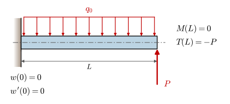
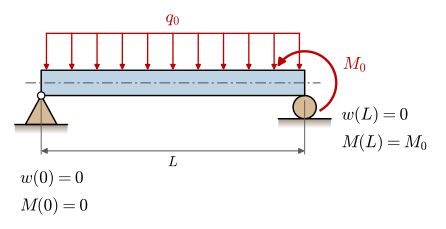
Two examples show how the conditions are read off a drawing, Figure 8.16.9. The cantilever in Figure 8.16.9 (a) is clamped at \(x = 0\), which prescribes the deflection and the slope, and free at \(x = L\), where nothing prevents the motion and so the moment and the shear are prescribed instead. No couple acts at the tip, so \(M(L) = 0\). The shear equals the tip load with the sign that 8.16.12 gives it: the shear force runs from \(T(L)\) just inside the end to zero beyond it, and a jump of \(+P\) for the upward force leaves \(T(L) = -P\). The simply supported beam in Figure 8.16.9 (b) has a deflection of zero at both supports, a moment of zero at the pinned end and a moment equal to the applied couple at the other, \(M(L) = M_0\) for an anticlockwise \(M_0\).

Example 1: A cantilever under its own distributed load

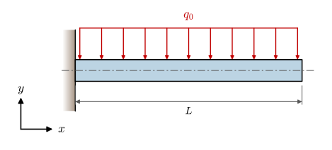
A cantilever of length \(L\) is clamped at \(x = 0\) and free at \(x = L\), carrying a uniformly distributed downward load of magnitude \(q_0\), as in Figure 8.16.10. Determine the deflection, and the tip deflection in particular.

The clamp fixes the deflection and the slope, and the free end carries no moment and no shear. With \(q = -q_0\) for the downward load the model is

\[ \begin{aligned} EI\,\frac{d^4 w}{dx^4} &= -q_0 \\ w(0) = w'(0) &= 0, \qquad M(L) = T(L) = 0 \end{aligned} \]

x, L, EI = sp.symbols('x L EI', positive=True)
q_0, E_s, I_s = sp.symbols('q_0 E I', positive=True)
w = sp.Function('w')

general = sp.dsolve(sp.Eq(E_s*I_s*sp.diff(w(x), x, 4), -q_0), w(x)).rhs
constants = sorted(general.free_symbols - {x, L, E_s, I_s, q_0}, key=lambda s: s.name)

M_expr = E_s*I_s*sp.diff(general, x, 2)
T_expr = E_s*I_s*sp.diff(general, x, 3)

bcs = [general.subs(x, 0),               # w(0) = 0
       sp.diff(general, x).subs(x, 0),   # w'(0) = 0
       M_expr.subs(x, L),                # M(L) = 0
       T_expr.subs(x, L)]                # T(L) = 0

sol = sp.solve(bcs, constants, dict=True)[0]
w_sol = sp.simplify(general.subs(sol))

ltx(r"w(x) &=", w_sol,
    r"\\ w(L) &=", sp.simplify(w_sol.subs(x, L)), aligned=True)

The tip deflection is \(-q_0 L^4/(8EI)\), negative because the beam sags in the direction the load pushes it, and matching the tabulated elementary case. The fourth power of the length is the reason cantilevers are so sensitive to their span: doubling the reach of an overhang increases its droop sixteenfold.

The whole ladder 8.16.14 follows by differentiation, so the shear and moment diagrams cost nothing extra.

theta_sol = sp.diff(w_sol, x)
M_sol = E_s*I_s*sp.diff(w_sol, x, 2)
T_sol = E_s*I_s*sp.diff(w_sol, x, 3)

ltx(r"\theta(x) &=", sp.simplify(theta_sol),
    r"\\ M(x) &=", sp.simplify(M_sol),
    r"\\ T(x) &=", sp.simplify(T_sol), aligned=True)

Both diagrams are exact and both make sense at a glance. The moment is largest in magnitude at the clamp, where it equals \(-q_0L^2/2\), the moment of the whole load about the support. The shear at the clamp is \(q_0 L\), the entire applied load, positive because the clamp pushes up on the left end of the beam, and both fall to zero at the free tip as the boundary conditions demanded.

Piecewise beams and matching conditions

8.16.13 assumes that \(q(x)\) is a smooth function of position, and real beams rarely oblige. A point load, an intermediate support, a step in cross section or an applied couple all break the beam into segments, within each of which the load is smooth but across which the solution is not.

The remedy is to write one differential equation per segment and to join the solutions with matching conditions, which the Swedish literature calls skarvvillkor. Each additional segment brings four more constants and therefore needs four more conditions, and the interface supplies exactly four. Two are kinematic: the beam does not break apart and does not develop a kink, so the deflection and the slope are continuous. Two are static: the internal moment and shear are continuous except for any concentrated moment or force applied at the joint, which enters as a jump.

For a joint at \(x = a\) carrying a downward point load \(P\) and no applied couple, the four conditions are

\[ \begin{array}{ll} w_1(a) = w_2(a) & \text{no separation}\\[4pt] w_1'(a) = w_2'(a) & \text{no kink}\\[4pt] M_1(a) = M_2(a) & \text{no applied couple}\\[4pt] T_1(a) - T_2(a) = P & \text{shear jumps by the point load} \end{array} \tag{8.16.16}\]

The last line is the one to check, on a simply supported beam of span \(L\) with a central point load that should deflect \(PL^3/(48EI)\). Both segments are unloaded and both ends pinned,

\[ \begin{aligned} EI\,\frac{d^4 w_i}{dx^4} &= 0, \quad i = 1, 2 \\ w_1(0) = M_1(0) &= 0, \qquad w_2(L) = M_2(L) = 0 \end{aligned} \]

with 8.16.16 at \(a = L/2\).

P = sp.symbols('P', positive=True)
w1f, w2f = sp.Function('w_1'), sp.Function('w_2')

gen1 = sp.dsolve(sp.Eq(E_s*I_s*sp.diff(w1f(x), x, 4), 0), w1f(x)).rhs
gen2 = sp.dsolve(sp.Eq(E_s*I_s*sp.diff(w2f(x), x, 4), 0), w2f(x)).rhs

C_1 = sorted(gen1.free_symbols - {x, E_s, I_s}, key=lambda s: s.name)
gen2 = gen2.subs({c: sp.Symbol('D' + c.name[1:]) for c in C_1})
C_2 = sorted(gen2.free_symbols - {x, E_s, I_s}, key=lambda s: s.name)

M_1, M_2 = E_s*I_s*sp.diff(gen1, x, 2), E_s*I_s*sp.diff(gen2, x, 2)
T_1, T_2 = E_s*I_s*sp.diff(gen1, x, 3), E_s*I_s*sp.diff(gen2, x, 3)

a = L/2
equations = [gen1.subs(x, 0), M_1.subs(x, 0),                        # pinned at 0
             gen2.subs(x, L), M_2.subs(x, L),                        # pinned at L
             (gen1 - gen2).subs(x, a),                               # continuity of y
             (sp.diff(gen1, x) - sp.diff(gen2, x)).subs(x, a),       # continuity of slope
             (M_1 - M_2).subs(x, a),                                 # continuity of moment
             (T_1 - T_2).subs(x, a) - P]                             # shear jump

sol = sp.solve(equations, C_1 + C_2, dict=True)[0]
w_mid = sp.simplify(gen1.subs(sol).subs(x, a))

ltx(r"w\!\left(\tfrac{L}{2}\right) =", w_mid)

The result is \(-PL^3/(48EI)\), downward and of exactly the tabulated magnitude, so the sign convention in 8.16.16 is the right one.

Example 2: A propped cantilever with an interior load

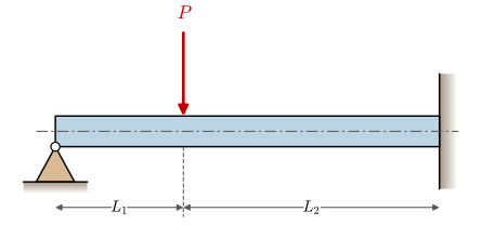
We now solve a case that no elementary table covers. A beam is pinned at \(x = 0\), clamped at the far end, and carries a downward point load \(P\) where its two segments meet, at \(x = L_1\). The second segment has length \(L_2\), as in Figure 8.16.11. The structure is statically indeterminate, so equilibrium alone cannot find the reactions and the deflection must be solved for first.

L_1, L_2 = sp.symbols('L_1 L_2', positive=True)

gen1 = sp.dsolve(sp.Eq(E_s*I_s*sp.diff(w1f(x), x, 4), 0), w1f(x)).rhs
gen2 = sp.dsolve(sp.Eq(E_s*I_s*sp.diff(w2f(x), x, 4), 0), w2f(x)).rhs
C_1 = sorted(gen1.free_symbols - {x, E_s, I_s}, key=lambda s: s.name)
gen2 = gen2.subs({c: sp.Symbol('D' + c.name[1:]) for c in C_1})
C_2 = sorted(gen2.free_symbols - {x, E_s, I_s}, key=lambda s: s.name)

M_1, M_2 = E_s*I_s*sp.diff(gen1, x, 2), E_s*I_s*sp.diff(gen2, x, 2)
T_1, T_2 = E_s*I_s*sp.diff(gen1, x, 3), E_s*I_s*sp.diff(gen2, x, 3)
L_tot = L_1 + L_2

equations = [gen1.subs(x, 0), M_1.subs(x, 0),                        # pinned at x = 0
             gen2.subs(x, L_tot), sp.diff(gen2, x).subs(x, L_tot),   # clamped at the far end
             (gen1 - gen2).subs(x, L_1),
             (sp.diff(gen1, x) - sp.diff(gen2, x)).subs(x, L_1),
             (M_1 - M_2).subs(x, L_1),
             (T_1 - T_2).subs(x, L_1) - P]

sol = sp.solve(equations, C_1 + C_2, dict=True)[0]
w_1 = sp.simplify(gen1.subs(sol))
w_2 = sp.simplify(gen2.subs(sol))

ltx(r"w_1(x) =", w_1)

With the symbolic solution in hand we insert a specific design. Take a square steel section \(100 \times 100~\text{mm}\), so that \(I = bh^3/12\) and the extreme fibre sits at \(c = 50~\text{mm}\), with \(L_1 = 1000~\text{mm}\), \(L_2 = 2000~\text{mm}\) and \(P = 1000~\text{N}\).

values = {E_s: 210e3, I_s: 100**4/12, P: 1000.0, L_1: 1000.0, L_2: 2000.0}
c_fibre = 50.0

pieces = []
for w_i, (x_a, x_b) in [(w_1, (sp.Integer(0), L_1)), (w_2, (L_1, L_tot))]:
    pieces.append(dict(
        w=sp.lambdify(x, w_i.subs(values), 'numpy'),
        th=sp.lambdify(x, sp.diff(w_i, x).subs(values), 'numpy'),
        M=sp.lambdify(x, (E_s*I_s*sp.diff(w_i, x, 2)).subs(values), 'numpy'),
        T=sp.lambdify(x, (E_s*I_s*sp.diff(w_i, x, 3)).subs(values), 'numpy'),
        span=(float(x_a.subs(values)), float(x_b.subs(values)))))

def sample(key):
    xs, vs = [], []
    for p in pieces:
        xi = np.linspace(*p['span'], 200)
        vi = np.asarray(p[key](xi), dtype=float) * np.ones_like(xi)
        xs.append(xi); vs.append(vi)
    return np.concatenate(xs), np.concatenate(vs)

x_v, w_v = sample('w')
_,   M_v = sample('M')
_,   T_v = sample('T')
sigma_v = M_v * c_fibre / values[I_s]

ltx(r"w_{\max} &=", float(np.min(w_v)), r"~\text{mm}",
    r"\\ M_{\max} &=", float(np.max(np.abs(M_v))), r"~\text{Nmm}",
    r"\\ \sigma_{\max} &=", float(np.max(np.abs(sigma_v))), r"~\text{MPa}", aligned=True)

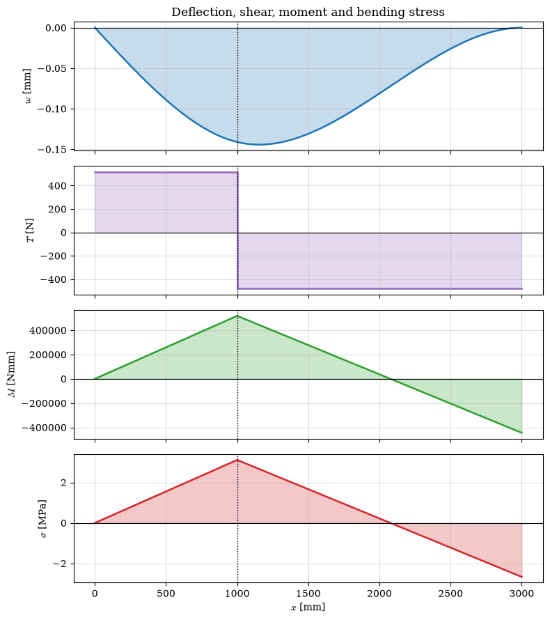
The largest deflection is \(0.14~\text{mm}\) downward and the largest bending stress is \(3.1~\text{MPa}\), so this section is enormously oversized for the load, which is what we would expect from a \(100~\text{mm}\) square carrying a kilonewton. Plotting the four diagrams together shows the structure of the solution.

fig, axes = plt.subplots(4, 1, figsize=(8, 9), sharex=True)

for a, v, lbl, col in zip(axes, (w_v, T_v, M_v, sigma_v),
                          (r"$w$ [mm]", r"$T$ [N]", r"$M$ [Nmm]", r"$\sigma$ [MPa]"),
                          ('C0', 'C4', 'C2', 'C3')):
    a.plot(x_v, v, color=col, lw=1.8)
    a.fill_between(x_v, 0, v, color=col, alpha=0.25)
    a.axhline(0, color='k', lw=0.8)
    a.axvline(float(values[L_1]), color='k', ls=':', lw=1)
    a.set_ylabel(lbl)
    a.grid(True, alpha=0.4)

axes[-1].set_xlabel(r"$x$ [mm]")
axes[0].set_title("Deflection, shear, moment and bending stress")
plt.tight_layout()
plt.show()

The shear is piecewise constant, as it must be when no distributed load acts, and it jumps by exactly \(P\) at the joint. The moment is piecewise linear, peaks at the joint where the shear changes sign, and is negative at the clamp because the beam curves the other way there. The bending stress is the moment scaled by \(c/I\), so it is the moment diagram in different units, and it passes through zero at the inflection point where the curvature reverses. That point is where the top surface of the beam stops being in compression and starts being in tension, which matters when the two surfaces are made of different materials or when only one of them is welded.

Example 3: A cantilever with several loads

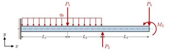
A beam taken from the finite element literature [1, Example 10.1] shows how far the piecewise approach goes without any change of method. The cantilever in Figure 8.16.13 is clamped at \(x = 0\) and free at \(x = L_1 + L_2 + L_3\), with \(L_1 = L_3 = 4~\text{m}\) and \(L_2 = 3~\text{m}\), and its bending stiffness is \(EI = 10^4~\text{Nm}^2\). A downward line load \(q_0 = 1~\text{N/m}\) covers the first two spans. The point loads are \(P_1 = 10~\text{N}\) downward at \(x = L_1\), \(P_2 = 5~\text{N}\) upward at \(x = L_1 + L_2\) and \(P_3 = 20~\text{N}\) downward at the tip, where an anticlockwise couple \(M_3 = 20~\text{Nm}\) also acts. Determine the deflection and the internal forces.

The loads split the beam into three segments, with joints at \(a = L_1\) and \(b = L_1 + L_2\) and the free end at \(L = L_1 + L_2 + L_3\). Each segment obeys 8.16.13,

\[ EI\,\frac{d^4 w_i}{dx^4} = -q_0, \quad i = 1, 2, \qquad EI\,\frac{d^4 w_3}{dx^4} = 0 \]

with four constants of its own. The clamp, 8.16.16 at the joints with \(P_1\) down and \(P_2\) up, and the loaded free end of Figure 8.16.9 give the twelve conditions

\[ \begin{aligned} w_1(0) &= 0, \quad w_1'(0) = 0 \\ w_1(a) &= w_2(a), \quad w_1'(a) = w_2'(a), \quad w_1''(a) = w_2''(a) \\ EI\,\bigl(w_1'''(a) - w_2'''(a)\bigr) &= P_1 \\ w_2(b) &= w_3(b), \quad w_2'(b) = w_3'(b), \quad w_2''(b) = w_3''(b) \\ EI\,\bigl(w_2'''(b) - w_3'''(b)\bigr) &= -P_2 \\ EI\,w_3''(L) &= M_3, \quad EI\,w_3'''(L) = P_3 \end{aligned} \]

q_0, P_1, P_2, P_3, M_3 = sp.symbols('q_0 P_1 P_2 P_3 M_3', real=True)
L_1, L_2, L_3 = sp.symbols('L_1 L_2 L_3', positive=True)
x_a, x_b, x_c = L_1, L_1 + L_2, L_1 + L_2 + L_3        # the two joints and the free end

# one elastic line per segment, q positive upward, each with four constants of its own
w_seg, C_seg = [], []
for i, q_i in enumerate((-q_0, -q_0, 0)):
    w_f = sp.Function(f'w_{i + 1}')
    general = sp.dsolve(sp.Eq(EI*sp.diff(w_f(x), x, 4), q_i), w_f(x)).rhs
    consts = sorted(general.free_symbols - {x, EI, q_0}, key=lambda s: s.name)
    fresh = sp.symbols(f'C_{i + 1}1:{i + 1}5')
    w_seg.append(general.subs(dict(zip(consts, fresh))))
    C_seg += fresh

th_seg = [sp.diff(w_i, x) for w_i in w_seg]
M_seg = [EI*sp.diff(w_i, x, 2) for w_i in w_seg]
T_seg = [EI*sp.diff(w_i, x, 3) for w_i in w_seg]

equations = [w_seg[0].subs(x, 0), th_seg[0].subs(x, 0)]              # clamped at x = 0
for j, (x_j, jump) in enumerate(((x_a, -P_1), (x_b, P_2))):          # P_1 down, P_2 up
    equations += [(w_seg[j] - w_seg[j + 1]).subs(x, x_j),
                  (th_seg[j] - th_seg[j + 1]).subs(x, x_j),
                  (M_seg[j] - M_seg[j + 1]).subs(x, x_j),
                  (T_seg[j + 1] - T_seg[j]).subs(x, x_j) - jump]     # the shear jumps by the load
equations += [M_seg[2].subs(x, x_c) - M_3,                           # the couple at the free end
              T_seg[2].subs(x, x_c) - P_3]                           # the tip load, downward

sol = sp.solve(equations, C_seg, dict=True)[0]
w_seg = [sp.expand(w_i.subs(sol)) for w_i in w_seg]
M_seg = [sp.expand(m.subs(sol)) for m in M_seg]
T_seg = [sp.expand(t.subs(sol)) for t in T_seg]

ltx(r"T(0) &=", sp.factor(T_seg[0].subs(x, 0)),
    r"\\ M(0) &=", sp.collect(sp.expand(M_seg[0].subs(x, 0)), [P_1, P_2, P_3, q_0]), aligned=True)

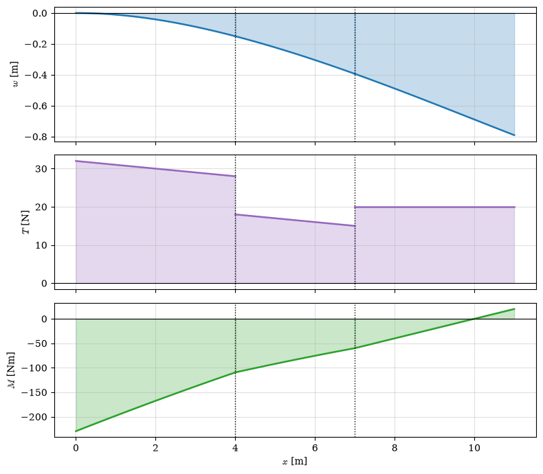
The two reactions at the clamp check against statics. The shear at the clamp is the vertical reaction, the sum of all the loads, \(q_0(L_1 + L_2) + P_1 - P_2 + P_3\), and the moment there balances the moments of the loads and the couple about the clamp. With the numbers of the example the shear at the clamp is \(7 + 10 - 5 + 20 = 32~\text{N}\) upward. The deflection and the slope at the second joint and at the tip are the nodal unknowns that the two-element finite element model of the original example solves for, there called \(w_2\), \(\theta_2\), \(w_3\) and \(\theta_3\). That model returns exactly these values, because its cubic elements reproduce the elastic line exactly at the nodes of a beam with constant \(EI\).

values = {q_0: 1, P_1: 10, P_2: 5, P_3: 20, M_3: 20, L_1: 4, L_2: 3, L_3: 4, EI: 1e4}

ltx(r"T(0) &=", T_seg[0].subs(x, 0).subs(values), r"~\text{N}",
    r"\\ w(L_1 + L_2) &=", w_seg[1].subs(x, x_b).subs(values), r"~\text{m}",
    r"\\ w'(L_1 + L_2) &=", sp.diff(w_seg[1], x).subs(x, x_b).subs(values),
    r"\\ w(L) &=", w_seg[2].subs(x, x_c).subs(values), r"~\text{m}",
    r"\\ w'(L) &=", sp.diff(w_seg[2], x).subs(x, x_c).subs(values),
    aligned=True, precision=4)

spans = ((0, x_a), (x_a, x_b), (x_b, x_c))
fig, axes = plt.subplots(3, 1, figsize=(8, 7), sharex=True)
for a_k, seg, lbl, col in zip(axes, (w_seg, T_seg, M_seg),
                              (r"$w$ [m]", r"$T$ [N]", r"$M$ [Nm]"), ('C0', 'C4', 'C2')):
    for f, (x0, x1) in zip(seg, spans):
        x0, x1 = float(sp.sympify(x0).subs(values)), float(sp.sympify(x1).subs(values))
        xs = np.linspace(x0, x1, 100)
        vs = sp.lambdify(x, f.subs(values), 'numpy')(xs)*np.ones_like(xs)
        a_k.plot(xs, vs, color=col, lw=1.8)
        a_k.fill_between(xs, 0, vs, color=col, alpha=0.25)
    for x_j in (x_a, x_b):
        a_k.axvline(float(x_j.subs(values)), color='k', ls=':', lw=1)
    a_k.axhline(0, color='k', lw=0.8)
    a_k.set_ylabel(lbl)
    a_k.grid(True, alpha=0.4)
axes[-1].set_xlabel(r"$x$ [m]")
plt.tight_layout()
plt.show()

Transverse shear stress

The Euler-Bernoulli kinematics produced a strain tensor with a single non-zero entry, so it predicts \(\varepsilon_{xy} = 0\) and hence, through \(\tau = G\gamma\), a transverse shear stress of exactly zero. Yet 8.16.12 plainly contains a shear force \(T\), and a force cannot be transmitted by a stress that is zero. The two statements contradict each other.

The contradiction is a consequence of the perpendicularity assumption, which forbids the cross section from shearing while the equilibrium of the beam requires it to. The standard resolution is to accept the kinematics for computing the bending stress and to obtain the shear stress from equilibrium instead. Take a slice of length \(\Delta x\) and cut it horizontally at some height, keeping the portion above the cut. The axial stress 8.16.10 acts on both ends of that portion, and because the moment changes across the slice the two are not equal. The imbalance must be carried by a shear stress \(\sigma_{yx}\) on the horizontal cut.

Writing the two axial resultants and the shear force on the horizontal face,

\[ \begin{aligned} F_1 &= \iint -\frac{M + \Delta M}{I}\, y\, dy\, dz \\ F_2 &= \iint \frac{M}{I}\, y\, dy\, dz \\ F_3 &= \sigma_{yx}\,\Delta x\, b \end{aligned} \]

where \(b\) is the width of the section at the height of the cut, equilibrium in the axial direction gives \(F_1 + F_2 + F_3 = 0\), which reduces to

\[ \iint -\frac{\Delta M}{I}\, y\, dy\, dz - \sigma_{yx}\,\Delta x\, b = 0 \]

Using \(\Delta M \approx (dM/dx)\,\Delta x = T \Delta x\) from 8.16.12 and cancelling \(\Delta x\) leaves

\[ \boxed{\tau = \sigma_{xy} = \sigma_{yx} = -\frac{T Q}{I b}}, \qquad Q := \iint y\, dy\, dz \tag{8.16.17}\]

where \(Q\) is the first moment of the area lying beyond the cut, taken about the neutral axis. The symmetry \(\sigma_{xy} = \sigma_{yx}\) that we proved in Chapter 8.7 is what allows the horizontal shear computed here to be read as the vertical shear on the cross section.

The distribution is instructive. At the top and bottom surfaces the area beyond the cut vanishes, so \(Q = 0\) and the shear stress is zero, as it must be on a free surface. At the neutral axis \(Q\) is largest, so the shear stress peaks there, exactly where the bending stress vanishes. For a rectangular section the profile is parabolic with a peak magnitude of \(\tfrac{3}{2}T/A\), fifty percent above the average.

xi, T_sym = sp.symbols('xi T', real=True)

# first moment of the area above the cut at height xi, about the neutral axis
Q_rect = b * sp.integrate(y, (y, xi, h_sec/2))
tau_rect = sp.simplify(-T_sym*Q_rect/(I_rect*b))               # @eq-shear-stress-beam

ltx(r"Q(\xi) &=", sp.simplify(Q_rect),
    r"\\ \tau(\xi) &=", tau_rect,
    r"\\ \tau(0) &=", sp.simplify(tau_rect.subs(xi, 0)), aligned=True)

With \(A = bh\) the peak magnitude is \(\tfrac{3}{2}T/A\) as claimed, and the minus sign is that of 8.16.17. In a slender beam the bending stress is much larger than this, which is why shear rarely governs the design of a long beam and often governs a short deep one.

The Timoshenko-Ehrenfest beam

The contradiction in the previous section is resolved properly by weakening the kinematic assumption. Keep the requirement that cross sections remain plane, but drop the requirement that they remain perpendicular to the neutral axis. The rotation of the cross section then becomes an independent function \(\psi\), related to the slope of the axis by

\[ \psi = w' + \varphi \]

where \(\varphi\) is the additional shear rotation. The displacement field 8.16.3 becomes

\[ \bm u = \begin{bmatrix} -y\,\psi \\ w \\ 0 \end{bmatrix} \tag{8.16.18}\]

and the same \(\bm\varepsilon = \tfrac12(\nabla\bm u + \nabla\bm u^\mathsf{T})\) applied to it now yields a strain tensor with a shear entry that no longer cancels.

x, y, z = sp.symbols('x y z', real=True)     # the coordinates again; x was reused for the examples
XX = sp.Matrix([x, y, z])
psi = sp.Function('psi')(x)
w_t = sp.Function('w')(x)

uu_t = sp.Matrix([-y*psi, w_t, 0])
grad_t = uu_t.jacobian(XX)
eps_t = sp.simplify((grad_t + grad_t.T)/2)

ltx(r"\nabla\bm u =", grad_t, r",\qquad \bm\varepsilon =", eps_t)

The axial strain is now \(\varepsilon_{xx} = -y\,d\psi/dx\), driven by the gradient of the section rotation rather than by the curvature of the axis, and the shear strain is

\[ 2\varepsilon_{xy} = \frac{dw}{dx} - \psi = -\varphi =: -\gamma \]

Integrating the stresses over the cross section as before gives the two internal force relations

\[ M = EI\frac{d\psi}{dx}, \qquad T = kAG\gamma \tag{8.16.19}\]

in which \(k\) is a shear correction factor. It is needed because the assumption of a plane cross section forces the shear stress to be uniform through the depth, whereas 8.16.17 says it is parabolic. The factor \(k\) smears the real distribution into an equivalent uniform one. Asking that the uniform shear stress \(T/(kA)\) store the same strain energy as the parabolic distribution of 8.16.17 gives \(k = 5/6\) for a rectangle. Cowper [2] derived \(k\) from the three-dimensional equations of elasticity instead and found \(k = 10(1+\nu)/(12+11\nu)\) for a rectangle, \(0.85\) for \(\nu = 0.3\), together with values for other sections. It is not an exact quantity, and different authors derive different values from different equivalence criteria.

Substituting 8.16.19 into the slice equilibrium 8.16.12 gives the governing pair

\[ \begin{aligned} EI\frac{d^3\psi}{dx^3} &= q \\ \frac{dw}{dx} &= \psi - \frac{EI}{kAG}\frac{d^2\psi}{dx^2} \end{aligned} \tag{8.16.20}\]

The first equation is solved for \(\psi\) and the second then integrated for \(w\), which introduces a fourth constant, so the Timoshenko beam still needs four boundary conditions. The deflection comes out as the Euler-Bernoulli answer plus a shear correction proportional to \(EI/(kAG)\); Wang, Reddy and Lee [3] give these relations between the two theories for the common beams and plates.

That group is the whole story. Write it as

\[ \frac{EI}{kAG L^2} \sim \frac{E}{G}\cdot\frac{I}{A L^2} \sim \frac{E}{G}\left(\frac{r}{L}\right)^2 \]

where \(r = \sqrt{I/A}\) is the radius of gyration of the section, a length of the order of its depth. Since \(E/G = 2(1+\nu) \approx 2.6\) by 8.9.5, the correction is a few times the square of the depth-to-span ratio. A beam ten times longer than it is deep gets a correction of a few percent and the Euler-Bernoulli model is entirely adequate. A beam three times longer than it is deep gets a correction approaching thirty percent, and a beam as deep as it is long is not a beam at all and should be modelled as a two-dimensional continuum.

When the beam model applies

Every result in this chapter descends from 8.16.3, so every result inherits its limitations. The model assumes that the cross section moves rigidly, which fails near a point where load is introduced, near a support, near a hole and near an abrupt change of section, because in those regions the cross section warps. Saint-Venant’s principle, Section 8.3.9, says that the disturbance decays within a distance of the order of the section depth, so the beam solution is accurate everywhere except in short zones around the discontinuities. Those zones are exactly where a finite element model earns its cost, and they are where the stress concentrations of a real design live.

The model also assumes bending in one plane about a principal axis of the section. Loading a section obliquely, or loading an unsymmetric section at all, couples bending about the two axes and, for open thin-walled sections, couples bending to torsion as well.

What we have gained is worth the restrictions. A partial differential equation for a vector field over a volume became an ordinary differential equation for a scalar on a line, solvable in closed form, differentiable into every quantity a designer needs, and cheap enough to put inside an optimisation loop. That trade, a kinematic assumption in exchange for a dimensional reduction, is the pattern behind every structural theory, and recognising it as a special case of the continuum model of Chapter 8.9 rather than as a separate subject is what makes the pattern visible.

The beam configurator

Available at mechanics.ju.se/marimo/beams, the configurator solves the elastic line for a beam on any number of supports, with point loads, couples and a trapezoidal distributed load on every segment, for a choice of cross section and with either theory. It draws the deformed beam with its support reactions, the bending and shear stresses and the diagrams. Its examples are the elementary cases of Björk’s formula book [4], each compared with the book’s formulas, and choosing the Timoshenko-Ehrenfest theory for a short, deep beam shows the shear angle of the previous section directly.

Further reading

Dahlberg [5] treats the same beam theory in Swedish, with many worked examples, and Adeeb’s open online textbook [6] covers the same ground in English. The elementary cases that designers look up, a cantilever or a simply supported beam under point loads, couples and distributed loads, are tabulated with their reactions, moments, deflections and rotations in Björk’s formula book [4]. The beam configurator above solves every one of them, compares its results with the book’s formulas, and solves as easily the combinations the tables leave out. Where the beam model stops applying, the finite element method takes over; Ottosen and Petersson [7] introduce it from the same continuum model.