“On ne dirait pas qu’il y a un travail produit, lorsqu’il y a seulement une force appliquée à un point immobile, comme dans une machine en équilibre; on n’appliquerait pas non plus l’expression de travail à un déplacement opéré sans aucune résistance vaincue.”
“We would not say that work has been produced when there is only a force applied at a motionless point, as in a machine in equilibrium; nor would we apply the word work to a displacement made with no resistance overcome.”
— Gaspard-Gustave de Coriolis, Du calcul de l’effet des machines, 1829
In Particle kinetics every problem ended in a differential equation in time, and we integrated it to get the whole motion. Many questions do not need the whole motion. How fast is the collar moving when it reaches the bottom of the guide? How fast does a falling counterweight hit the ground? The answer depends on where the body is, not on when it gets there, and Newton’s second law integrated along the path answers it directly.
We start with a problem solved the way we already know, with a free body diagram and Newton’s second law. Integrating that equation along the path turns the forces into energies, and the result is a balance between two states of the system, before and after. The balance can then be written down from the start, by modelling the energy of the system instead of the forces on it.
The energy balance has a second use, as important as the first: it checks a solution we already have. When we integrate an equation of motion numerically, nothing guarantees that the result is right. A system without friction or damping keeps its total energy, so the energy computed from the numerical solution must stay constant, and how far it drifts measures the error of the integration. We use it that way in this chapter and in every chapter that follows.
The chapter ends with power, the rate at which work is done, which is what a motor has to deliver.
Example 1: A collar on a curved guide
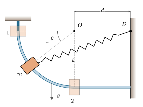
A collar of mass \(m = 3\) kg slides without friction on a guide bent into a quarter circle of radius \(r = 0.6\) m, followed by a straight horizontal part (Figure 7.3.1). A spring of stiffness \(k = 350\) N/m connects the collar to the point \(D\) on the wall, at the height of the centre \(O\) and \(d = 0.6\) m to the right of it. The unstretched length of the spring is \(d\). The collar is released from rest at \(1\), where the spring is horizontal. Find its speed \(v_2\) when it reaches \(2\), the bottom of the curve.
Figure 7.3.1: The collar slides on the guide from \(1\) to \(2\), pulled by the spring anchored at \(D\). The angle \(\theta\) is measured from the horizontal through \(O\).
Step 1 - Free body diagram and equations of motion
The collar moves on a circle about \(O\), the same circle as the packages of Example 9 in Particle kinetics, and we use the same natural coordinates. With \(O\) at the origin, \(x\) to the right and \(y\) up,
with \(\bm e_n\) pointing to the centre and \(\bm e_t\) along the path in the direction of increasing \(\theta\). The accelerations along them are \(a_t = r\ddot\theta\) and \(a_n = r\dot\theta^2\).
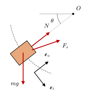
Three forces act on the collar (Figure 7.3.2): the weight \(\bm F_W = -mg\,\bm e_y\), the normal force \(\bm N = N\bm e_n\) from the smooth guide, and the spring force. The spring runs from the collar to \(D = (d, 0)\),
The normal force has no tangential component, so the tangential equation holds the motion and the normal equation holds the contact force.
Figure 7.3.2: The collar at the angle \(\theta\), with its weight, the normal force and the spring force.
Code
t = sp.symbols('t', positive=True)m, r, d, k, g = sp.symbols('m r d k g', positive=True)N = sp.symbols('N', real=True)th, thd, thdd = sp.symbols(r'theta \dot\theta \ddot\theta', real=True)ee_n = sp.Matrix([sp.cos(th), sp.sin(th)])ee_t = sp.Matrix([sp.sin(th), -sp.cos(th)])rr_C =-r*ee_nrr_CD = sp.Matrix([d, 0]) - rr_Cell = sp.sqrt(d**2+2*d*r*sp.cos(th) + r**2) # |r_CD|, simplified by handFF_W = sp.Matrix([0, -m*g])FF_s = k*(ell - d)*rr_CD/ellFF_N = N*ee_neqs = [sp.Eq((FF_W + FF_s + FF_N).dot(ee_t), m*r*thdd), sp.Eq((FF_W + FF_s + FF_N).dot(ee_n), m*r*thd**2)]sol = sp.solve(eqs, [thdd, N], dict=True)[0]sol = {key: sp.simplify(val) for key, val in sol.items()}
Solving the two equations for \(\ddot\theta\) and \(N\) gives
\[ \begin{aligned}
N &= \dot\theta^{2} m r + \dfrac{d^{2} k \cos{\left(\theta \right)}}{\sqrt{d^{2} + 2 d r \cos{\left(\theta \right)} + r^{2}}} + \dfrac{d k r}{\sqrt{d^{2} + 2 d r \cos{\left(\theta \right)} + r^{2}}} - d k \cos{\left(\theta \right)} + g m \sin{\left(\theta \right)} - k r \\[9.0pt]
\ddot\theta &= \dfrac{- \dfrac{d^{2} k \sin{\left(\theta \right)}}{\sqrt{d^{2} + 2 d r \cos{\left(\theta \right)} + r^{2}}} + d k \sin{\left(\theta \right)} + g m \cos{\left(\theta \right)}}{m r}
\end{aligned} \]
Step 2 - The equation of motion
The spring’s tangential component simplifies. Since \(\bm r_{CD}\cdot\bm e_t = (d + r\cos\theta)\sin\theta - r\sin\theta\cos\theta = d\sin\theta\), only the offset \(d\) of the anchor gives the spring a component along the guide, and the tangential equation becomes
At the release the spring is horizontal and pulls straight towards the centre line, so only gravity starts the motion. Further down, the stretched spring pulls the collar forward as well. 7.3.1 is nonlinear in \(\theta\) through both terms, and \(\ell\) depends on \(\theta\) too.
Step 3 - Time integration
We integrate 7.3.1 with the Euler-Cromer method of Particle kinetics. With \(\omega = \dot\theta\) and the time step \(\Delta t\),
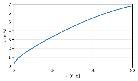
The collar reaches the bottom after 0.35 s at 6.82 m/s. The plot shows the speed against the angle. It rises fastest just after the release, where the guide is nearly vertical and gravity acts almost entirely along the guide, and more slowly towards \(2\), where the guide turns horizontal and the spring has given up most of its stretch.
The time history was not asked for. The question is about a position, so we can use the chain rule \(a\,ds = v\,dv\) of 6.3.3 and integrate along the path instead. The collar moves the arc length \(ds = r\,d\theta\), and its tangential acceleration is \(a_t = r\ddot\theta\), so
with \(\ddot\theta(\theta)\) from 7.3.1 and \(v_1 = 0\). The gravity term integrates to \(gr\). The spring term looks harder, but \(\ell\) is the substitution that does it: differentiating \(\ell^2 = d^2 + 2dr\cos\theta + r^2\) gives \(\ell\,d\ell = -dr\sin\theta\,d\theta\), and the spring term becomes
\[ \begin{aligned}\frac{1}{2}v_2^2 &=- \dfrac{d k \left(d - \sqrt{d^{2} + r^{2}}\right)}{m} + g r\\ v_2 &=6.824~\text{m/s}\end{aligned} \]
The path integral gives \(v_2 = 6.824\) m/s, the result of the time integration, with no time step and no time history. Look at the three terms of 7.3.2. The left side depends only on the speed at \(2\). On the right, \(mgr\) depends only on the drop in height, and each spring term only on the spring length at one end of the path. Nothing in the result remembers the shape of the guide between \(1\) and \(2\). That is the observation the rest of the chapter is built on.
From Newton to energy
We repeat Step 4 for any path, term by term, without solving for the acceleration first. Newton’s second law for the collar, written with everything on one side, is
\[
\bm F_W + \bm F_s + \bm N - m\bm a = \bm 0 .
\]
Its dot product with the displacement \(d\bm r\) along the path, integrated from \(1\) to \(2\), is still zero,
\[
\int_1^2 \bm F_W\cdot d\bm r + \int_1^2 \bm F_s\cdot d\bm r + \int_1^2 \bm N\cdot d\bm r - \int_1^2 m\bm a\cdot d\bm r = 0 ,
\tag{7.3.3}\]
and each of the four integrals can be done on its own.
The normal force is perpendicular to the guide and \(d\bm r\) is along it, so \(\bm N\cdot d\bm r = 0\). The guide steers the collar but does not speed it up.
The weight is constant. With \(y\) measured upwards, \(\bm F_W\cdot d\bm r = -mg\,dy\), and
The spring force points along \(\bm r_{CD}\), and as the collar moves by \(d\bm r\) the spring length changes by \(d\ell = -\bm r_{CD}\cdot d\bm r/\ell\). So \(\bm F_s\cdot d\bm r = -k(\ell - d)\,d\ell\), and with the stretch \(\delta = \ell - d\),
The inertia term uses \(d\bm r = \bm v\,dt\) and \(\bm a = d\bm v/dt\). Then \(m\bm a\cdot d\bm r = m\bm v\cdot d\bm v = d\bigl(\tfrac{1}{2}m\,\bm v\cdot\bm v\bigr)\), and
Each of the three surviving integrals is the change of a function of the state: the height, the stretch and the speed. We name those functions the gravitational potential energy\(V_g = mgy\), the elastic potential energy\(V_e = \tfrac{1}{2}k\delta^2\) and the kinetic energy\(T = \tfrac{1}{2}mv^2\). Putting the initial values on the left and the final values on the right, 7.3.3 becomes
The total mechanical energy \(E = T + V_g + V_e\) is the same at \(1\) and at \(2\), and by the same argument at every point in between. Whatever the collar loses in height and in spring stretch it gains in speed.
Work and potential energy
The integral of a force along the path of its point of application is the work the force does,
\[
U_{1\to2} = \int_1^2 \bm F\cdot d\bm r ,
\]
measured in joules, \(1~\text{J} = 1~\text{N}\cdot\text{m}\). Only the component of the force along the path does work, which is Coriolis’s point in the epigraph: a force at a point that does not move does none, and neither does a force perpendicular to the motion. The normal force of a smooth fixed guide, the reaction at a fixed pin and the force on a wheel rolling without slip all do no work.
A moment does work through a rotation. A couple \(M\) acting on a body that turns by \(d\theta\) does the work \(dU = M\,d\theta\), so
Force and displacement belong together, and so do moment and rotation: each product is a work. We call such pairs work-conjugate. Solid mechanics adds stress and strain as a third pair.
The weight and the spring force share one property: their work depends only on the end points of the path. Such forces are conservative, and each has a potential energy \(V\) whose decrease is the work done. For a displacement along \(x\) or a rotation \(\theta\),
\[
F = -\frac{dV}{dx} , \qquad M = -\frac{dV}{d\theta} ,
\]
so a conservative force is the slope of its potential energy, and a moment is the slope with respect to an angle. The two potentials of this chapter are
with \(h\) the height above a reference level we are free to choose and \(\delta\) the stretch or compression of the spring from its unstretched length.
Friction, drag, dampers and the force of a motor are not conservative: their work depends on the path or on how fast it is travelled. We collect their work in \(U'_{1\to2}\) and keep it on the left with the initial state,
where \(V\) is the sum of all potential energies. When \(U'_{1\to2} = 0\) this is 7.3.4. For a system of several bodies the energies are summed over the bodies. The forces between them do no net work when they are rigidly connected, pinned together, or joined by an inextensible rope over ideal pulleys, because each such force does equal and opposite work on the two bodies it connects.
Example 2: The collar, modelled with energy
We solve Example 1 again, this time without a free body diagram. The guide does no work and there is no friction, so \(U'_{1\to2} = 0\) and 7.3.4 applies. We put the reference level for \(V_g\) at \(2\) and write each energy in the two states of Figure 7.3.1.
In state \(1\) the collar is at rest, a height \(r\) above \(2\), and the spring is stretched from \(d\) to \(\ell_1 = r + d\):
Three lines give the speed that took four steps with Newton’s second law. The energy route is short because it never meets the normal force, which does no work, and never asks when the collar arrives. The same two facts are its limits. It gives the speed at \(2\) but not the time to get there, and not the force the guide carries.
The two routes combine well. With \(v_2\) known from energy, the normal equation of Step 1 at \(\theta = \pi/2\) gives the contact force at \(2\), where \(\bm e_n = \bm e_y\) points up to \(O\) and the spring pulls along \(\bm r_{CD}/\ell_2 = [d,\ r]^\mathsf{T}/\ell_2\),
The guide pushes up on the collar at \(2\) with 201 N, almost seven times its weight, because it turns a collar moving at 6.8 m/s on a radius of 0.6 m.
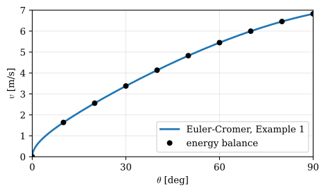
Nothing in the balance is special to the end point. At any angle \(\theta\) the collar is \(r\sin\theta\) below its start and the spring has the length \(\ell(\theta)\), so the same balance gives the speed along the whole guide,
The energy balance lies on the numerical solution at every angle, which checks the integration, the energies and the claim that the guide does no work.
Energy as a check on a time integration
The comparison above needed the energy balance solved for \(v(\theta)\). A simpler check needs no solving at all. At every step \(i\) of the time integration we know \(\theta_i\) and \(\omega_i = \dot\theta_i\), so we can compute the total energy of the collar, with the reference level at \(2\),
The exact solution keeps \(E\) at its initial value \(E_0\), so the relative drift
\[
\varepsilon_i = \frac{E_i - E_0}{E_0}
\]
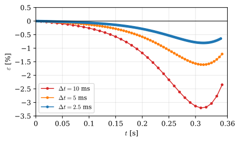
measures the error of the numerical solution, without knowing the exact one. We run the Euler-Cromer integration of Example 1 with three time steps, each half the previous one.
The computed energy falls by up to 3.2 % with \(\Delta t = 10\) ms, 1.6 % with 5 ms and 0.8 % with 2.5 ms. Halving the time step halves the error, the signature of a first-order method, and the 10 µs step used in Example 1 keeps the drift below \(4\cdot 10^{-5}\). A drift that does not shrink with the time step points to an error in the model itself, a wrong sign or a missing term, and no refinement will remove it.
TipIn industry: the energy balance as a check
Explicit crash and impact codes such as LS-DYNA can report the energy balance of the whole model, split into kinetic, internal, contact and hourglass energy and the external work. It is important to check that the total stays consistent with the initial energy and the external work, and that the purely numerical terms stay small. What counts as acceptable depends on the model, but a run that fails the check deserves a closer look, however convincing its animation.
Example 3: The log on the ramp, with friction
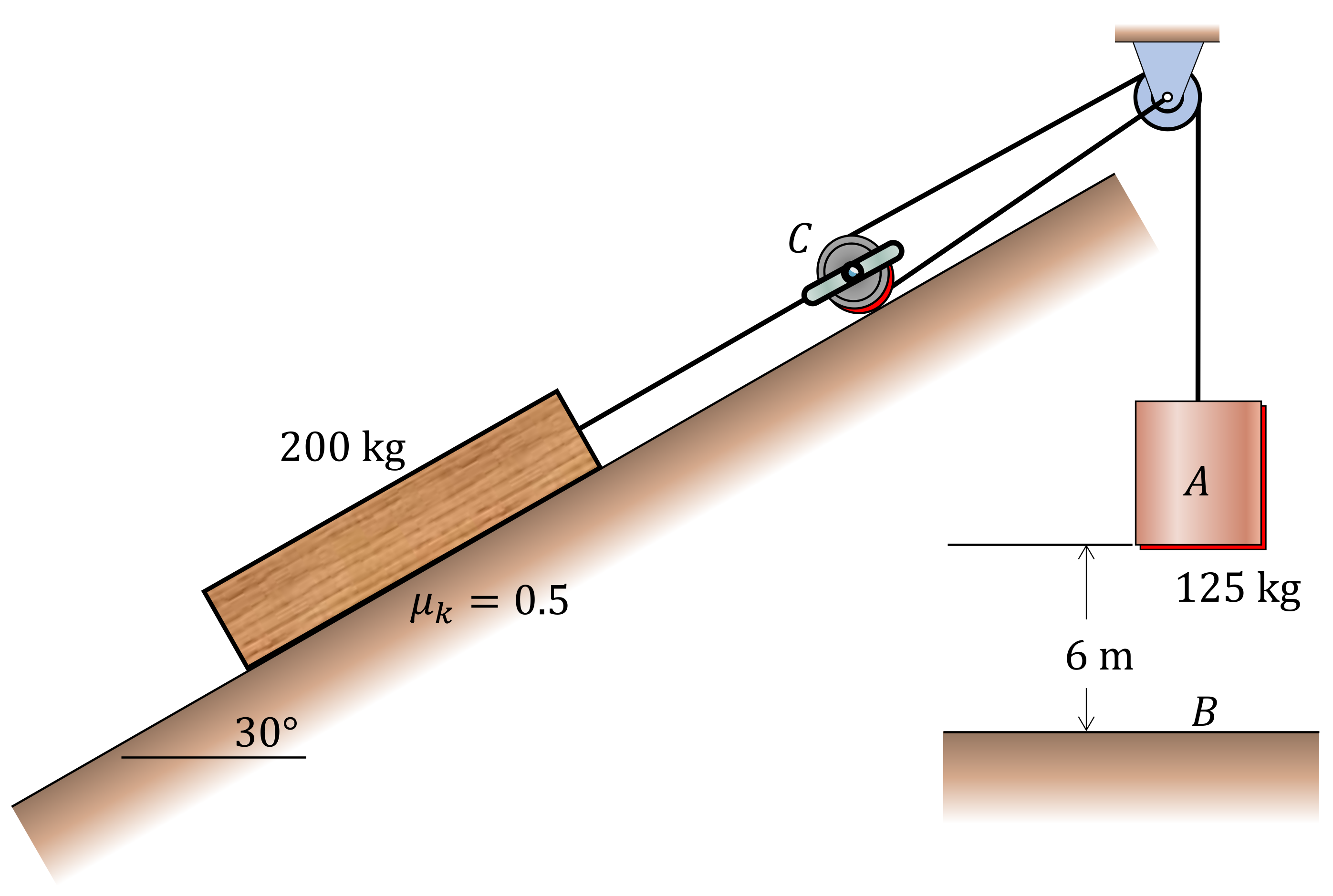
Example 3 in Particle kinetics found the impact speed of a counterweight that pulls a log up a ramp through a pulley system (Figure 7.3.3). The data are \(m_1 = 200\) kg for the log, \(m_2 = 125\) kg for the counterweight, a ramp angle \(\theta = 30^\circ\), kinetic friction \(\mu_k = 0.5\) between log and ramp, and a drop of \(h = 6\) m. The system starts from rest. We find the impact speed \(v_A\) again, with energy.
Figure 7.3.3: The log, pulled up the ramp by the rope around its pulley, and the counterweight that falls \(h\) to the ground.
We take the log and the counterweight together as one system. The rope is inextensible and the pulleys are ideal, so the rope tension does no net work on the system. The rope fixes the kinematics, \(s_A = 2s_C\) and \(v_A = 2v_C\): while the counterweight falls \(h\), the log climbs \(h/2\) along the ramp and rises \((h/2)\sin\theta\).
Friction is the one non-conservative force. It acts against the log’s motion over the distance \(h/2\), so its work is negative,
The normal force comes from Newton’s second law perpendicular to the ramp, where the log does not accelerate. The energy balance alone cannot give it, so a friction problem always needs a piece of a free body diagram.
With the reference levels at the start, 7.3.5 reads
The impact speed is 4.618 m/s, as in Particle kinetics. The counterweight releases 7.36 kJ of potential energy as it falls. The log stores 2.94 kJ of it as height, friction turns 2.55 kJ into heat, and the remaining 1.87 kJ is the kinetic energy of the two bodies at impact. The kinetic energy \(\tfrac{1}{2}(m_1/4 + m_2)v_A^2\) also shows the effective inertia that Particle kinetics found, \(m_1 + 4m_2\) seen from the log, here seen from the counterweight.
Power
The energy balance tells us how much work a motor must do, but not how fast. A motor that lifts a load slowly and one that lifts it quickly do the same work; the second one delivers it in less time. The rate of doing work is the power,
\[
P = \frac{dU}{dt} = \bm F\cdot\frac{d\bm r}{dt} = \bm F\cdot\bm v ,
\]
measured in watts, \(1~\text{W} = 1~\text{J/s}\). For a moment acting on a turning shaft, \(dU = M\,d\theta\) gives
\[
P = M\omega .
\]
A shaft at a given power can carry a large moment at low speed or a small moment at high speed. A gearbox trades one for the other and leaves the power unchanged, apart from its losses.
No machine passes on all the power it receives. Friction in bearings, gears and screws turns part of it into heat, and the ratio of the power out to the power in is the efficiency,
For a chain of machines, such as a motor driving a gearbox driving a drum, the efficiencies multiply.
NoteFreedom units: the horsepower
James Watt sold steam engines to brewers and mill owners who until then had used horses, so he rated his engines by the number of horses they replaced. The story usually told is that he watched a mill horse walk round a mill wheel of 12 ft radius, 144 times an hour, pulling with 180 pounds-force. That is \(180 \cdot 2\pi \cdot 12 \cdot 2.4 \approx 32\,600\) ft·lbf per minute, which Watt rounded to 33 000 ft·lbf/min, or 550 ft·lbf/s. In SI units this mechanical horsepower is 745.7 W.
The metric horsepower (Pferdestärke, PS, or hästkraft, hk) is defined as lifting 75 kg by one metre in one second, \(75~\text{kgf}\cdot\text{m/s} = 735.5\) W. The two differ by about 1.4 %, enough to make engine ratings from different countries disagree.
Example 4: A winch on a ramp
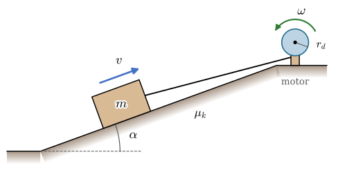
A winch hauls a crate of mass \(m = 150\) kg up a ramp inclined at \(\alpha = 20^\circ\) at the constant speed \(v = 0.5\) m/s (Figure 7.3.4). The coefficient of kinetic friction between crate and ramp is \(\mu_k = 0.3\). The cable runs parallel to the ramp onto a drum of radius \(r_d = 0.1\) m, driven by an electric motor through a gearbox; motor and gearbox together have the efficiency \(\eta = 0.75\). Find the power the motor draws, and the speed and moment at the drum.
Figure 7.3.4: The crate is hauled up the ramp at constant speed by a cable wound onto the drum of the winch.
The crate does not accelerate, so the forces along and perpendicular to the ramp balance. With the cable force \(F\),
\[
F - mg\sin\alpha - \mu_k N = 0 , \qquad N - mg\cos\alpha = 0
\quad\Longrightarrow\quad
F = mg\,(\sin\alpha + \mu_k\cos\alpha) .
\]
The power the cable delivers to the crate is \(P_{\text{out}} = Fv\). The cable leaves the drum at the speed \(v\), so the drum turns at \(\omega = v/r_d\) under the moment \(M = F r_d\), and \(M\omega = Fv\) is the same power. The motor draws
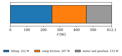
\[ \begin{aligned}F &=918.1~\text{N}\\ P_{\text{out}} = Fv &=459.1~\text{W}\\ \omega &=5~\text{rad/s} \approx47.8~\text{rpm}\\ M = F r_d &=91.81~\text{N}\cdot\text{m}\\ P_{\text{in}} &=612.1~\text{W}\end{aligned} \]
The motor draws 612 W to deliver 459 W to the crate, and the drum turns slowly, at 48 rpm, under a moment of 92 N·m. Every second the crate rises \(v\sin\alpha\) and gains \(mgv\sin\alpha = 252\) J of potential energy, and friction turns \(\mu_k mg v\cos\alpha = 207\) J into heat. Their sum is the 459 W of the cable. The kinetic energy of the crate does not change, so none of the power goes into speed.
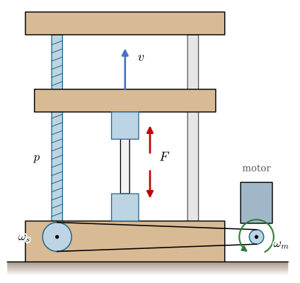
A tensile testing machine pulls a specimen apart by moving its crosshead up a vertical ball screw (Figure 7.3.5). The machine is to pull with \(F = 50\) kN at crosshead speeds up to \(v = 500\) mm/min. The screw has the lead \(p = 10\) mm, so one turn moves the crosshead 10 mm, and its efficiency is \(\eta_s = 0.9\). A toothed belt with the ratio \(i = \omega_m/\omega_s = 3\) and the efficiency \(\eta_b = 0.95\) connects the motor to the screw. Find the moment and speed the motor must deliver, and its power.
Figure 7.3.5: The crosshead rides on the screw of lead \(p\), which the motor turns through a belt. The specimen between the grips carries the force \(F\).
In one turn the screw moment \(M_s\) does the work \(2\pi M_s\), of which the fraction \(\eta_s\) reaches the crosshead, and the crosshead does the work \(Fp\) against the specimen. The work balance per turn gives the screw moment,
\[
\eta_s\,2\pi M_s = F p
\quad\Longrightarrow\quad
M_s = \frac{F p}{2\pi\,\eta_s} .
\]
The screw turns \(v/p\) times per unit time, so \(\omega_s = 2\pi v/p\). The belt speeds up the motor by \(i\) and takes the fraction \(1 - \eta_b\) of the power on the way, so the motor runs at
The crosshead does 417 W of work on the specimen at full force and full speed, and the motor must deliver 487 W. A motor turning at only 150 rpm with 31 N·m is large and expensive. Electric motors give their power most cheaply at a few thousand rpm, so real machines put a gearbox between motor and screw. With a total ratio of \(i = 60\) the motor runs at 3000 rpm and needs only \(M_m = M_s/(i\,\eta) \approx 1.6\) N·m. The power stays the same, because it is fixed by the force, the speed and the losses: \(P_m = Fv/\eta\), whatever the transmission. Choosing the ratio is choosing where on that power the moment and the speed lie.
The work balance per turn of the screw, \(\eta_s\,2\pi M_s = Fp\), is a first use of an idea the chapter on virtual work develops: the force relation of a mechanism follows from comparing the work done at its input and output, without the forces inside it.
Further reading
Meriam, Kraige and Bolton treat work, energy and power for particles in chapter 3 of their Dynamics[1], with many more problems.