import sympy as sp
from mechanicskit import la

F_A, F_B, m, g = sp.symbols('F_A F_B m g')

def ee(theta_deg):
    """Unit direction vector from angle in degrees."""
    theta = sp.rad(theta_deg)
    return sp.Matrix([sp.cos(theta), sp.sin(theta), 0])

FF_A = F_A * ee(15)
FF_B = F_B * ee(120)
FF_G = sp.Matrix([0, -m*g, 0])5.4 Static Equilibrium
Newton’s second law states that the resultant force on a body equals its mass times acceleration, \(\sum \bm F = m\bm a\). Euler’s second law gives the rotational counterpart, \(\sum \bm M = I\bm \alpha\). In statics we study bodies at rest or in uniform motion, so \(\bm a = 0\) and \(\bm \alpha = 0\). The governing equations reduce to
\[ \sum \bm F = 0, \quad \sum \bm M = 0 \tag{5.4.1}\]
Newton’s third law tells us that every force has an equal and opposite reaction. This is the reason we isolate bodies and draw free body diagrams: once we cut a body free from its surroundings, every contact and support becomes a force that we can account for.
That is all the theory there is. The rest is methodology and practice. The only path to understanding statics is by working examples.
Solution strategy
- What is known and unknown?
- Free body diagram
- Insert coordinate system
- Identify a suitable point for a moment equation
- \(\sum \bm M = 0\)
- \(\sum \bm F = 0\)
- Solve the equation system for the unknowns
- Analyze the results, plot, visualize
- Conclusion
Static determinacy
Before solving, always count unknowns and equations. In 2D a rigid body gives 3 independent equilibrium equations (2 force, 1 moment). In 3D it gives 6 (3 force, 3 moment). Each support contributes a certain number of unknown reaction components depending on its type (see the Free Body Diagram chapter).
If the number of unknowns equals the number of independent equations the system is statically determinate and can be solved by equilibrium alone. If there are more unknowns than equations the system is statically indeterminate and requires additional information about the deformation and material properties of the bodies. We will return to this in the Solid Mechanics part.
A multi-body system with \(n\) bodies gives \(3n\) equations in 2D (\(6n\) in 3D). The unknowns include both external reactions and internal joint forces at connections between bodies. The choice of support types is a modeling decision that directly affects whether the problem is determinate.
Example 1 – Sphere on smooth surfaces
A sphere with mass \(m\) rests against two smooth surfaces as shown below. We want to determine the normal forces at \(A\) and \(B\).
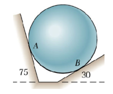
We insert a coordinate system at the center of the sphere and draw the free body diagram. Since the surfaces are smooth they can only exert normal forces. All forces pass through the center, so force equilibrium alone is sufficient.
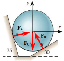
The contact surface at \(A\) has a normal direction at \(180° - 75° - 90° = 15°\) from the positive \(x\)-axis, and the surface at \(B\) has a normal at \(30° + 90° = 120°\). We define a unit direction vector \(\bm e(\theta) = [\cos\theta, \sin\theta, 0]^T\) and express each force as a magnitude times its direction.
eqn = sp.Eq(FF_A + FF_B + FF_G, sp.Matrix([0, 0, 0]))

sol = sp.solve(eqn, [F_A, F_B])
sol | la
\[ \begin{aligned} F_{A} &= \dfrac{\sqrt{2} g m}{1 + \sqrt{3}} \\[9.0pt] F_{B} &= g m \end{aligned} \]
Evaluating numerically, \(F_A \approx 0.52\,mg\) and \(F_B \approx 1.0\,mg\). The force at \(B\) carries nearly the full weight while \(A\) takes about half. This makes sense from the geometry: if we rotated the system \(30°\) clockwise, \(B\) would point straight up and carry all the weight, while \(A\) would vanish.
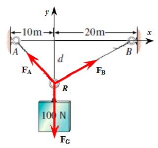
Example 2 – Wire tensions as a function of geometry
A 100 N weight hangs from a point \(R\) that is connected by wires to supports at \(A\) and \(B\). The distance \(d\) below the support line is a free parameter. We want to determine how the wire tensions vary with \(d\).
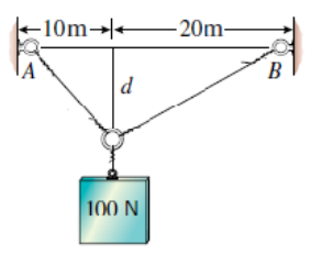
In contrast to the previous example where forces had known directions given by angles, here the forces act along lines between known points. We define position vectors for each point and compute the wire directions from the geometry.
F_A, F_B = sp.symbols('F_A F_B')
d = sp.symbols('d', positive=True) # to avoid abs in the solution

# Points
rr_A = sp.Matrix([-10, 0, 0])
rr_B = sp.Matrix([ 20, 0, 0])
rr_R = sp.Matrix([  0,-d, 0])

# Direction vectors from R toward supports
RA = rr_A - rr_R
RB = rr_B - rr_R

# Force vectors: magnitude times unit direction
FF_A = F_A * RA / RA.norm()
FF_B = F_B * RB / RB.norm()
FF_G = sp.Matrix([0, -100, 0])
eqn = sp.Eq(FF_A + FF_B + FF_G, sp.Matrix([0, 0, 0]))eqn | la(arraystretch=2.5)\[ {\def\arraystretch{2.5}\left[\begin{matrix}- \dfrac{10 F_{A}}{\sqrt{d^{2} + 100}} + \dfrac{20 F_{B}}{\sqrt{d^{2} + 400}}\\\dfrac{F_{A} d}{\sqrt{d^{2} + 100}} + \dfrac{F_{B} d}{\sqrt{d^{2} + 400}} - 100\\0\end{matrix}\right] = \left[\begin{matrix}0\\0\\0\end{matrix}\right]} \]
sol = sp.solve(eqn, [F_A, F_B])
sol | la
\[ \begin{aligned} F_{A} &= \dfrac{200 \sqrt{d^{2} + 100}}{3 d} \\[9.0pt] F_{B} &= \dfrac{100 \sqrt{d^{2} + 400}}{3 d} \end{aligned} \]
The solution is symbolic in \(d\). We can visualize how the tensions change as the hanging point drops.
Code
import matplotlib.pyplot as plt
from mechanicskit import fplot

fplot(sol[F_A], (d, 1, 30), label='$F_A$')
fplot(sol[F_B], (d, 1, 30), label='$F_B$')
plt.gca().set(xlabel='$d$ [m]', ylabel='Force [N]')
plt.legend()
plt.show()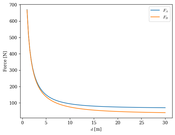
As \(d\) increases the wires become more vertical and the tensions approach reasonable values. As \(d \to 0\) the wires become nearly horizontal and the tensions blow up: a perfectly horizontal wire cannot support a vertical load. This is a fundamental insight that appears repeatedly in engineering.
We can utillize sympys limit function to compute the limits analytically, e.g., we let \(d\to 0\)
sp.limit(sol[F_A], d, 0) | la\[ {\def\arraystretch{1.0}\infty} \]
and with \(d\to \infty\)
sp.limit(sol[F_A], d, sp.oo) | la\[ {\def\arraystretch{1.0}\dfrac{200}{3}} \]
sp.limit(sol[F_B], d, sp.oo) | la\[ {\def\arraystretch{1.0}\dfrac{100}{3}} \]
Example 3 – Board carried by three people
A rectangular board with mass \(m\) is carried horizontally by three people. Each person can only exert a force in the positive \(z\)-direction. We want to determine how much each person lifts.
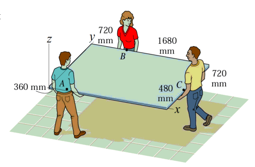
This is a three-dimensional problem. We place the origin at the lower-left corner and define position vectors for each person and for the center of gravity. Now both force and moment equilibrium are needed: three unknowns (\(F_{Az}\), \(F_{Bz}\), \(F_{Cz}\)) require three equations.
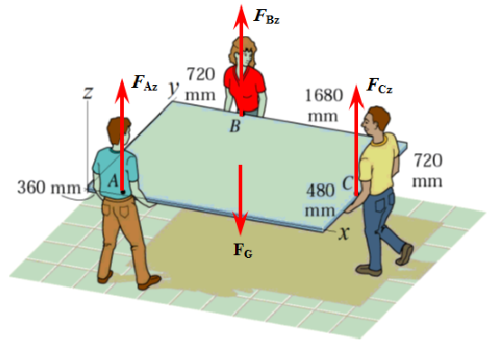
F_Az, F_Bz, F_Cz, mg = sp.symbols('F_Az F_Bz F_Cz mg', positive=True)

# Positions [mm]
rr_A = sp.Matrix([360, 0, 0]) / 1000        # convert to [m]
rr_B = sp.Matrix([720, 480+720, 0]) / 1000
rr_C = sp.Matrix([720+1680, 480, 0]) / 1000
rr_G = sp.Matrix([720+1680, 480+720, 0]) / 2000

# Forces (z-direction only)
FF_A = sp.Matrix([0, 0, F_Az])
FF_B = sp.Matrix([0, 0, F_Bz])
FF_C = sp.Matrix([0, 0, F_Cz])
FF_G = sp.Matrix([0, 0, -mg])
# Force equilibrium
N2 = sp.Eq(FF_A + FF_B + FF_C + FF_G, sp.Matrix([0, 0, 0]))
# Moment equilibrium about the origin
E2 = sp.Eq(
rr_A.cross(FF_A) + rr_B.cross(FF_B) + rr_C.cross(FF_C) + rr_G.cross(FF_G),
sp.Matrix([0, 0, 0])
)sol = sp.solve([N2, E2], [F_Az, F_Bz, F_Cz])
sol | la.evalf()\[ \begin{aligned} F_{Az} &= 0.2911 mg \\[9.0pt] F_{Bz} &= 0.3608 mg \\[9.0pt] F_{Cz} &= 0.3481 mg \end{aligned} \]
The solution expresses each lifting force as a fraction of the total weight \(mg\). The person closest to the center of gravity actually lifts the most, because the shortest lever arm requires the largest force to balance the moment about the other supports. The method is identical to the 2D case: define points, define forces, write \(\sum \bm F = 0\) and \(\sum \bm M = 0\), solve. The cross product in the moment equation handles the three-dimensional geometry automatically.
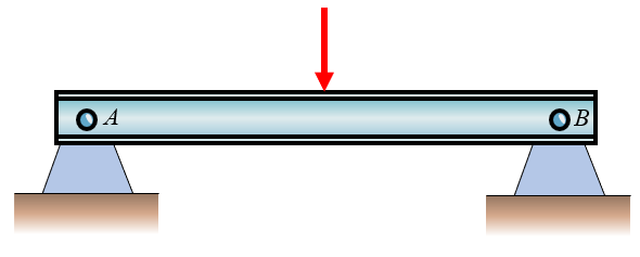
Example 4 – Static determinacy
We take the same beam loaded by a single force \(\bm F\) and change only the supports. The beam has length \(L\) and the force acts at \(L/2\). We set up the equilibrium equations for each case and observe what SymPy returns.
Case 1: Determinate (pin + roller)
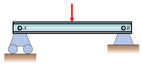
A pin at \(A\) gives two unknowns (\(R_{Ax}\), \(R_{Ay}\)) and a roller at \(B\) gives one (\(R_{By}\)). That is 3 unknowns and 3 equations.
from mechanicskit import ltx

L, F = sp.symbols('L F', positive=True)

# Case 1: pin at A (2 unknowns) + roller at B (1 unknown)
R_Ax, R_Ay, R_By = sp.symbols('R_Ax R_Ay R_By', real=True)

rr_A  = sp.Matrix([0, 0, 0])
rr_B  = sp.Matrix([L, 0, 0])
rr_F  = sp.Matrix([L/2, 0, 0])

RR_A = sp.Matrix([R_Ax, R_Ay, 0])
RR_B = sp.Matrix([0, R_By, 0])
FF   = sp.Matrix([0, -F, 0])

sumF = RR_A + RR_B + FF
sumM = rr_B.cross(RR_B) + rr_F.cross(FF)
\[ \sum \bm F = \left[\begin{matrix}R_{Ax}\\- F + R_{Ay} + R_{By}\\0\end{matrix}\right] = \bm 0 \]
\[ \sum \bm M = \left[\begin{matrix}0\\0\\- \frac{F L}{2} + L R_{By}\end{matrix}\right] = \bm 0 \]
sol1 = sp.solve([sumF, sumM], [R_Ax, R_Ay, R_By])
sol1 | la
\[ \begin{aligned} R_{Ax} &= 0 \\[9.0pt] R_{Ay} &= \dfrac{F}{2} \\[9.0pt] R_{By} &= \dfrac{F}{2} \end{aligned} \]
A unique solution: \(R_{Ax} = 0\), \(R_{Ay} = F/2\), \(R_{By} = F/2\). By symmetry both supports carry half the load. The beam is statically determinate.
Case 2: Indeterminate (pin + pin)
Both \(A\) and \(B\) are pins, giving 4 unknowns (\(R_{Ax}\), \(R_{Ay}\), \(R_{Bx}\), \(R_{By}\)) but still only 3 equations.
# Case 2: pin at A (2 unknowns) + pin at B (2 unknowns)
R_Ax, R_Ay, R_Bx, R_By = sp.symbols('R_Ax R_Ay R_Bx R_By', real=True)

RR_A = sp.Matrix([R_Ax, R_Ay, 0])
RR_B = sp.Matrix([R_Bx, R_By, 0])

sumF = RR_A + RR_B + FF
sumM = rr_B.cross(RR_B) + rr_F.cross(FF)
\[ \sum \bm F = \left[\begin{matrix}R_{Ax} + R_{Bx}\\- F + R_{Ay} + R_{By}\\0\end{matrix}\right] = \bm 0 \]
\[ \sum \bm M = \left[\begin{matrix}0\\0\\- \frac{F L}{2} + L R_{By}\end{matrix}\right] = \bm 0 \]
sol2 = sp.linsolve([sumF[0], sumF[1], sumM[2]],
                   (R_Ax, R_Ay, R_Bx, R_By))
sol2
\(\displaystyle \left\{\left( - R_{Bx}, \ \frac{F}{2}, \ R_{Bx}, \ \frac{F}{2}\right)\right\}\)
SymPy returns the solution in terms of \(R_{Bx}\), a free parameter. There are infinitely many solutions because equilibrium alone cannot determine how the horizontal reaction distributes between the two pins. This system is statically indeterminate and we would need to consider the deformation of the beam to find \(R_{Bx}\).
Code
sol2 = sp.solve([sumF[0], sumF[1], sumM[2]],
                 (R_Ax, R_Ay, R_Bx, R_By))
sol2 | la
\[ \begin{aligned} R_{Ax} &= - R_{Bx} \\[9.0pt] R_{Ay} &= \dfrac{F}{2} \\[9.0pt] R_{By} &= \dfrac{F}{2} \end{aligned} \]
Case 3: Under-constrained (roller + roller)
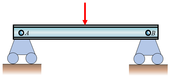
Both supports are rollers, giving only 2 unknowns (\(R_{Ay}\), \(R_{By}\)) for 3 equations.
# Case 3: roller at A (1 unknown) + roller at B (1 unknown)
R_Ay, R_By = sp.symbols('R_Ay R_By', real=True)

RR_A = sp.Matrix([0, R_Ay, 0])
RR_B = sp.Matrix([0, R_By, 0])
FF_3 = sp.Matrix([F, -F, 0])      # force with horizontal component F_x = F

sumF = RR_A + RR_B + FF_3
sumM = rr_B.cross(RR_B) + rr_F.cross(FF_3)
\[ \sum \bm F = \left[\begin{matrix}F\\- F + R_{Ay} + R_{By}\\0\end{matrix}\right] = \bm 0 \]
\[ \sum \bm M = \left[\begin{matrix}0\\0\\- \frac{F L}{2} + L R_{By}\end{matrix}\right] = \bm 0 \]
sol3 = sp.linsolve([sumF[0], sumF[1], sumM[2]], (R_Ay, R_By))
sol3
\(\displaystyle \emptyset\)
sp.linsolve returns the empty set: the system is inconsistent and there is no solution. Note that we used linsolve here rather than solve. If we hand the same equations to sp.solve asking only for \(R_{Ay}\) and \(R_{By}\), it silently throws away the \(x\)-equation (because it contains none of the requested unknowns) and reports the misleading answer \(R_{Ay}=R_{By}=F/2\). We can force sp.solve to behave correctly by adding the horizontal force component to the list of unknowns:
# Treat the horizontal force as an unknown so sp.solve cannot drop its equation
F_x = sp.Symbol('F_x', real=True)
FF_3 = sp.Matrix([F_x, -F, 0])
sumF = sp.Matrix([0, R_Ay, 0]) + sp.Matrix([0, R_By, 0]) + FF_3
sumM = rr_B.cross(sp.Matrix([0, R_By, 0])) + rr_F.cross(FF_3)

sp.solve([sumF, sumM], [R_Ay, R_By, F_x]) | la
\[ \begin{aligned} F_{x} &= 0 \\[9.0pt] R_{Ay} &= \dfrac{F}{2} \\[9.0pt] R_{By} &= \dfrac{F}{2} \end{aligned} \]
sp.solve is forced to set \(F_x=0\) to satisfy the \(x\)-equation, contradicting the nonzero horizontal load we applied. Either way the conclusion is the same: no equilibrium configuration exists. Two rollers cannot resist any horizontal load, so the beam would slide. This system is under-constrained: it is a mechanism, not a structure.
Note that with a purely vertical force the two-roller case does give a unique answer for the vertical reactions. The deficiency only becomes apparent when a horizontal load is present. This is why we must always check that the supports can resist loads in all directions that might arise, not just the ones in the current problem.
Remarks on determinacy
The counting of unknowns against equations is one of the most important modeling skills in mechanics. It determines whether a problem can be solved by equilibrium alone or whether we need additional physical laws (deformation, constitutive relations). In this course we restrict ourselves to statically determinate problems. The indeterminate case requires knowledge of how materials deform under load, which we treat in the Solid Mechanics part. Any course on the Finite Element Method (FEM/FEA) builds directly on this foundation: the concept of degrees of freedom, constraints, and how they relate to the solvability of a system is exactly the same, scaled up to thousands of elements.
For a multi-body example where the choice of support type determines whether the system is determinate, see Example 3 in the Equilibrium Examples chapter.
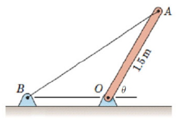
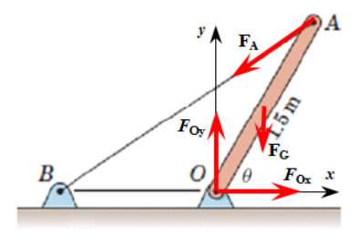
Example 5 – Rod held by a wire
A homogeneous rod of length 1.5 m and mass \(m\) is free to rotate about a pin at \(O\). A wire from the top of the rod at \(A\) to a fixed point \(B\) on the ground holds it in place. The geometry has two free parameters: the angle \(\theta\) between the rod and the horizontal, and the distance \(b\) from \(O\) to \(B\) along the negative \(x\)-axis. We want to determine the wire force and the reaction at \(O\) as functions of these parameters.
The pin at \(O\) contributes two reaction components \(R_x\) and \(R_y\), the wire contributes one unknown tension \(F_A\) along the line from \(A\) toward \(B\). With three unknowns and three equations (two force, one moment) the system is statically determinate. We take moments about \(O\), which eliminates the pin reactions from the moment equation.
theta, b, mg = sp.symbols('theta b mg', positive=True)
F_A, R_x, R_y = sp.symbols('F_A R_x R_y', real=True)

# Position vectors
rr_OA = 1.5 * sp.Matrix([sp.cos(theta), sp.sin(theta), 0])
rr_OB = sp.Matrix([-b, 0, 0])
rr_OG = rr_OA / 2

# Wire force at A pointing toward B
ee_AB = (rr_OB - rr_OA).normalized()
FF_A = F_A * ee_AB
FF_G = sp.Matrix([0, -mg, 0])
FF_O = sp.Matrix([R_x, R_y, 0])

sumF = FF_A + FF_G + FF_O
sumM = rr_OA.cross(FF_A) + rr_OG.cross(FF_G)
sol = sp.solve([sumF, sumM], [F_A, R_x, R_y])
sol | la.simplify().evalf(4)\[ \begin{aligned} F_{A} &= \dfrac{0.866 mg \left(0.3333 b^{2} + 1.0 b \cos{\left(\theta \right)} + 0.75\right)^{0.5}}{b \tan{\left(\theta \right)}} \\[9.0pt] R_{x} &= \dfrac{mg \left(0.5 b + 0.75 \cos{\left(\theta \right)}\right)}{b \tan{\left(\theta \right)}} \\[9.0pt] R_{y} &= \dfrac{mg \left(b + 0.75 \cos{\left(\theta \right)}\right)}{b} \end{aligned} \]
With two free parameters we can vary one at a time. First we fix the angle at \(\theta = 60°\) and sweep the wire attachment \(b\) from 0.5 m to 5 m.
Code
F_A_b = sol[F_A].subs({theta: sp.rad(60), mg: 1})
R_x_b = sol[R_x].subs({theta: sp.rad(60), mg: 1})
R_y_b = sol[R_y].subs({theta: sp.rad(60), mg: 1})

fplot(F_A_b, (b, 0.5, 5), label='$F_A(\\theta=60^\\circ)$')
fplot(R_x_b, (b, 0.5, 5), label='$R_x(\\theta=60^\\circ)$')
fplot(R_y_b, (b, 0.5, 5), label='$R_y(\\theta=60^\\circ)$')
plt.gca().set(xlabel='$b$ [m]', ylabel='$F / mg$')
plt.legend()
plt.show()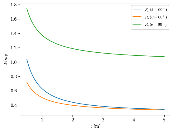
Then we fix the wire attachment at \(b = 1.5\) m and sweep the angle from \(0°\) to \(90°\).
Code
F_A_t = sol[F_A].subs({b: sp.Rational(3, 2), mg: 1})
R_x_t = sol[R_x].subs({b: sp.Rational(3, 2), mg: 1})
R_y_t = sol[R_y].subs({b: sp.Rational(3, 2), mg: 1})

fplot(F_A_t, (theta, sp.rad(5), sp.rad(89)), label='$F_A(b=1.5)$')
fplot(R_x_t, (theta, sp.rad(5), sp.rad(89)), label='$R_x(b=1.5)$')
fplot(R_y_t, (theta, sp.rad(5), sp.rad(89)), label='$R_y(b=1.5)$')
plt.gca().set(xlabel=r'Angle $\theta$ [rad]', ylabel='$F / mg$', ylim=[0, 5])
plt.legend()
plt.show()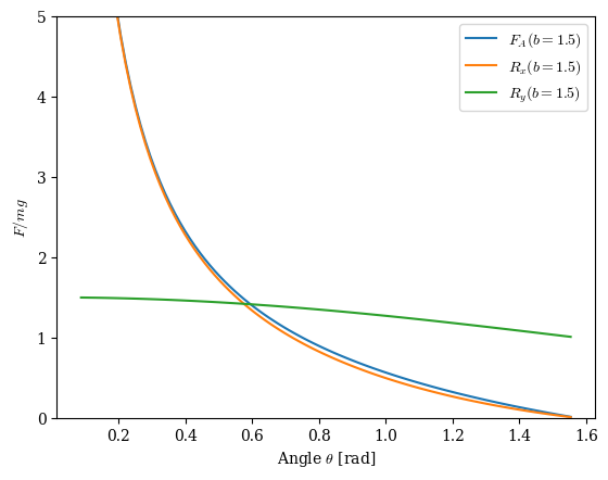
As \(\theta \to 90°\) the rod stands vertically and the weight acts directly above the pin. The horizontal reaction \(R_x\) vanishes, the vertical reaction \(R_y\) carries the full weight, and the wire force \(F_A\) drops to zero. The wire is no longer needed when the rod is balanced on its support, which is exactly the physical intuition we should expect from the geometry.
Example 6 – Light crane
A light crane is rigged according to the figure. The boom is pinned at the origin \(O\), supported by two wires (one from \(A\) to \(B\) and one from \(C\) to \(D\)), and carries a load \(F_L\) at a hook that travels along the boom at distance \(x\) from \(O\). We want to determine the wire tensions and the pin reaction at \(O\) as functions of \(x\), and then find the position that minimizes the magnitude of the pin reaction.
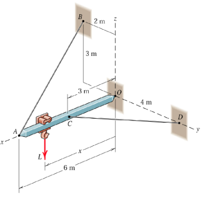
The pin at \(O\) contributes three reaction components, the two wires contribute one tension each, giving five unknowns. Force equilibrium gives three equations and moment equilibrium about \(O\) gives three more, but the moment about the boom axis vanishes identically because all forces and lever arms in this problem lie in planes containing the boom. That leaves five independent equations for five unknowns, so the system is determinate. Taking moments about \(O\) removes the pin reactions from the moment equation, leaving the wire tensions to be found first.
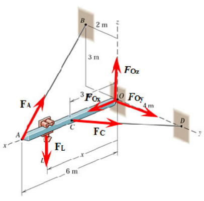
F_L, x = sp.symbols('F_L x', positive=True, real=True)
F_A, F_C = sp.symbols('F_A F_C', real=True)
F_Ox, F_Oy, F_Oz = sp.symbols('F_Ox F_Oy F_Oz', real=True)

# Position vectors [m]
rr_OA = sp.Matrix([6,  0, 0])     # boom tip
rr_OB = sp.Matrix([0, -2, 3])     # wire A anchor
rr_OC = sp.Matrix([3,  0, 0])     # wire C attachment on boom
rr_OD = sp.Matrix([0,  4, 0])     # wire C anchor
rr_OL = sp.Matrix([x,  0, 0])     # load position on boom

# Wire forces along the rope directions
ee_AB = (rr_OB - rr_OA).normalized()
ee_CD = (rr_OD - rr_OC).normalized()
FF_A = F_A * ee_AB
FF_C = F_C * ee_CD

# Pin reaction and load
FF_O = sp.Matrix([F_Ox, F_Oy, F_Oz])
FF_L = F_L * sp.Matrix([0, 0, -1])

sumF = FF_A + FF_C + FF_O + FF_L
sumM = rr_OA.cross(FF_A) + rr_OC.cross(FF_C) + rr_OL.cross(FF_L)
sol = sp.solve([sumF, sumM], [F_A, F_C, F_Ox, F_Oy, F_Oz])
sol | la.simplify()\[ \begin{aligned} F_{A} &= \dfrac{7 F_{L} x}{18} \\[9.0pt] F_{C} &= \dfrac{5 F_{L} x}{18} \\[9.0pt] F_{Ox} &= \dfrac{F_{L} x}{2} \\[9.0pt] F_{Oy} &= - \dfrac{F_{L} x}{9} \\[9.0pt] F_{Oz} &= \dfrac{F_{L} \left(6 - x\right)}{6} \end{aligned} \]
All five quantities scale linearly with the load \(F_L\), which is exactly what we expect from a linear statics problem. The interesting question is the magnitude of the pin reaction \(F_O = \sqrt{F_{Ox}^2 + F_{Oy}^2 + F_{Oz}^2}\) as a fraction of the load. We compute it symbolically and look for the position \(x\) that minimizes it.
F_O = sp.sqrt(sol[F_Ox]**2 + sol[F_Oy]**2 + sol[F_Oz]**2)
ratio = sp.simplify(F_O / F_L)
ratio | la
\[ {\def\arraystretch{1.0}\dfrac{\sqrt{94 x^{2} - 108 x + 324}}{18}} \]
x_min = sp.solve(sp.diff(ratio, x), x)[0]
ratio_min = sp.simplify(ratio.subs(x, x_min))
{sp.Symbol('x_{min}'): x_min, sp.Symbol(r'F_O/F_L|_{min}'): ratio_min} | la.evalf()
\[ \begin{aligned} x_{min} &= 0.5745 \\[9.0pt] F_O/F_L|_{min} &= 0.9509 \end{aligned} \]
Sweeping the load position \(x\) from \(0\) to \(6\) m shows how all five reaction quantities vary along the boom.
Code
fplot(sol[F_A].subs(F_L, 1),  (x, 0, 6), label='$F_A$')
fplot(sol[F_C].subs(F_L, 1),  (x, 0, 6), label='$F_C$')
fplot(sol[F_Ox].subs(F_L, 1), (x, 0, 6), label='$F_{Ox}$')
fplot(sol[F_Oy].subs(F_L, 1), (x, 0, 6), label='$F_{Oy}$')
fplot(sol[F_Oz].subs(F_L, 1), (x, 0, 6), label='$F_{Oz}$')
fplot(ratio,                  (x, 0, 6), label='$|F_O|/F_L$', linewidth=2.5)
plt.gca().set(xlabel='$x$ [m]', ylabel='Force / $F_L$')
plt.legend()
plt.show()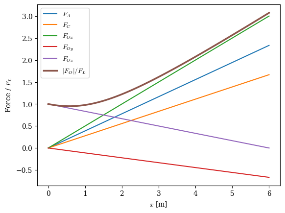
At \(x = 0\) the load sits directly above the origin and only the vertical component \(F_{Oz}\) is needed to support it, with both wires slack. As the hook moves outward both wire tensions grow linearly, the horizontal pin reactions \(F_{Ox}\) and \(F_{Oy}\) grow with it, and the vertical reaction shrinks because more of the load is carried by the wires. The ratio \(F_O / F_L\) has a clear minimum around \(x \approx 0.57\) m, which is the optimal hook position if we want to keep the bearing at \(O\) as lightly loaded as possible.