9.2 Parametric Involute Spur Gear in SolidWorks
“Involute teeth differ from the epicycloidal teeth … in having the entire side of the tooth, both face and flank, formed of a continuous curve.”
— Robert Willis, Principles of Mechanism, 1841
Gear teeth are usually drawn rather than derived. Most CAD tutorials approximate the flank with two or three tangent arcs, and most gear configurators generate the profile internally without stating whether what comes out is a true involute. The guides that do reach for the equation driven curve generally paste in a fixed expression without saying where it comes from, or leave enough of the surrounding sketch dimensioned by hand that the model stops rebuilding as soon as the tooth count changes.
We build the gear the other way round. Every dimension follows from the module \(m\), the tooth count \(N\) and the pressure angle \(\varphi\), the flank is a single equation driven curve that is an involute by construction, and the sketch topology is arranged so that it does not depend on \(N\). Changing the tooth count then rebuilds the model instead of breaking it. The motivation is partly academic, since a gear tooth is one of the few machine element surfaces whose shape is fixed by a kinematic requirement rather than chosen for convenience, and partly practical, since a model built this way can be checked and reused.
The chapter sets out the geometry of a tooth, then gives the SolidWorks procedure from an empty part to a finished gear, and finally derives the equations the procedure uses. A reader who only wants the model can stop after the SolidWorks procedure.
Anatomy of a gear tooth
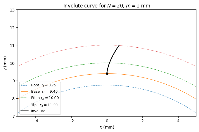
A spur gear is fixed by four concentric circles and one angle. The pitch circle of radius \(r_p = mN/2\) is where two meshing gears roll on one another without sliding, and it carries the definition of the module \(m\) as pitch diameter per tooth. The base circle of radius \(r_b = r_p\cos\varphi\) is the circle the involute unwinds from, with \(\varphi\) the pressure angle. The tip circle at \(r_a = m(N+2)/2\) and the root circle at \(r_f = r_p - 1.25\,m\) bound the tooth radially, the addendum reaching one module above the pitch circle and the dedendum \(1.25\) modules below it, the extra quarter module being the bottom clearance \(c_P = 0.25\,m\) that leaves room for the tip of the mating tooth. These proportions and the \(20°\) pressure angle are the standard basic rack tooth profile of ISO 53 [1]. All four are drawn in Figure 9.2.1.
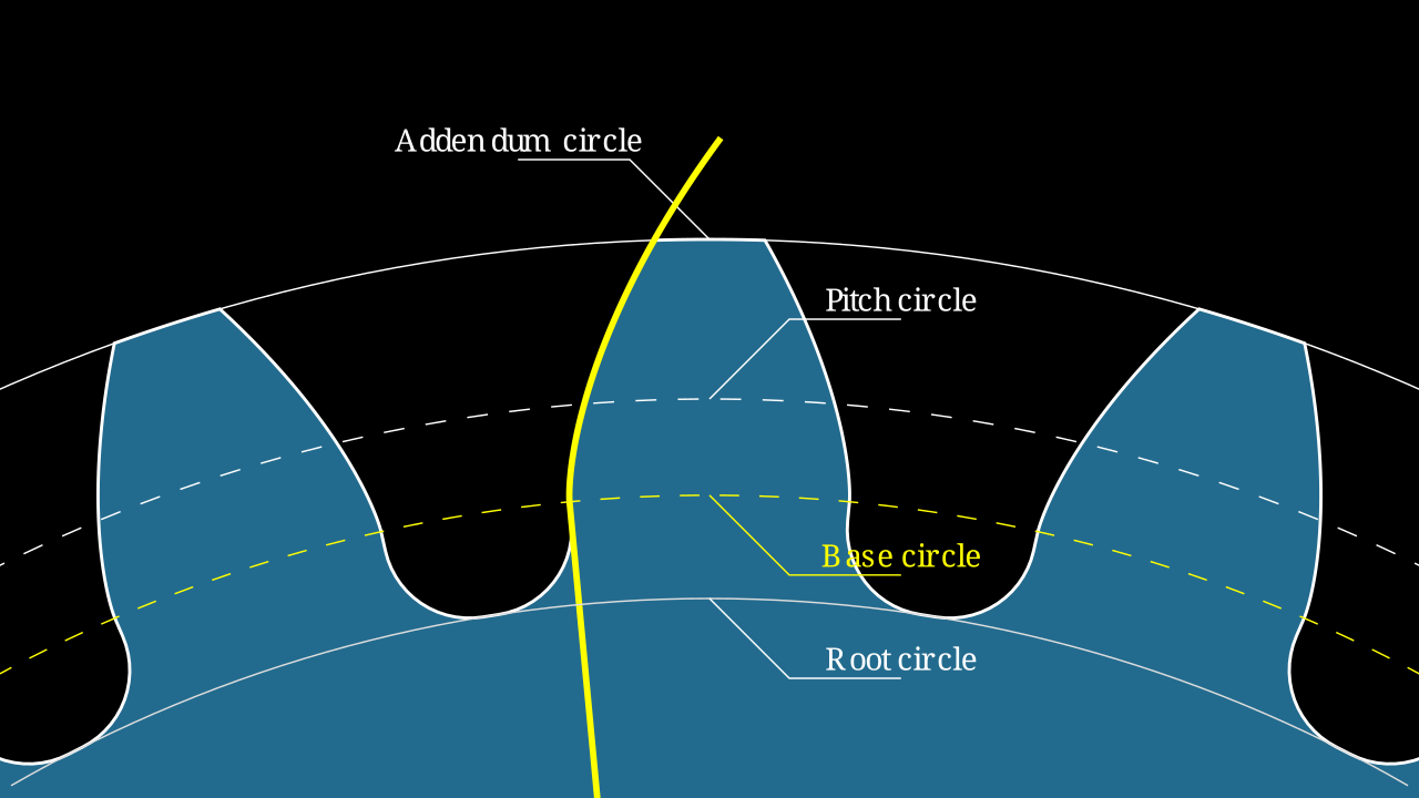
Whether the involute reaches all the way down to the root depends on the tooth count. Setting \(r_f = r_b\) and solving for \(N\) gives the crossover
\[ N = \frac{2.5}{1 - \cos\varphi} \tag{9.2.1}\]
which is \(41.5\) teeth at \(20°\). Below that the root circle lies inside the base circle, and the part of the flank between root and base is not an involute at all, because no involute exists there. Above it the involute covers the full flank and the two circles have swapped places. This single fact is what makes a naive parametric gear model fragile, and the flank curve deals with it.
The involute of a circle
The involute is the curve traced by the end of a taut string as it unwinds from a cylinder. Writing \(r\) for the radius of that cylinder and \(\alpha\) for the angle through which the string has unwound, the point on the curve is the tangency point on the circle plus the unwound length \(r\alpha\) measured along the tangent,
\[ \begin{bmatrix} x(\alpha) \\ y(\alpha) \end{bmatrix} = r \begin{bmatrix} \sin\alpha \\ \cos\alpha \end{bmatrix} + r\alpha \begin{bmatrix} -\cos\alpha \\ \sin\alpha \end{bmatrix} \tag{9.2.2}\]
At \(\alpha = 0\) the curve sits on the base circle itself, at the cusp, and as \(\alpha\) grows it spirals outward.
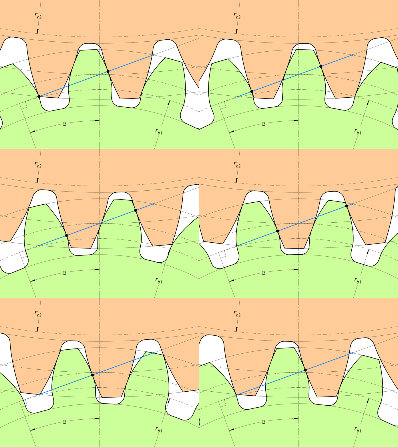
The property that matters for gearing is that the normal to the involute at every point passes through the tangency point on the base circle. Two involute flanks in contact therefore push on one another along a line that is fixed in space, the line of action, and the angular velocity ratio stays constant even when the centre distance is disturbed. That tolerance to centre distance error is why the involute displaced the cycloid during the nineteenth century and why it is now the only profile in general use [2].
Figure 9.2.2 shows what that means in practice: the contact point runs along the blue line, and it is the same line at every instant, whatever position the teeth are in.
Two quantities that follow from 9.2.2 are used repeatedly below. The radius reached at parameter \(\alpha\) is \(r = r_b\sqrt{1+\alpha^2}\). For the polar angle, reading the two components of 9.2.2 as the real and imaginary parts of one complex number gives
\[ (\cos\alpha + \alpha\sin\alpha) + i(\sin\alpha - \alpha\cos\alpha) = e^{i\alpha}(1 - i\alpha) \]
so the angle swept from the cusp is the argument of the right hand side,
\[ \psi(\alpha) = \alpha - \arctan\alpha \tag{9.2.3}\]
Evaluating 9.2.3 at the pitch circle, where \(\alpha_p = \sqrt{(r_p/r_b)^2 - 1} = \tan\varphi\), gives the involute function
\[ \operatorname{inv}\varphi = \tan\varphi - \varphi \tag{9.2.4}\]
which is \(0.8540°\) at \(\varphi = 20°\). Since the tooth count cancels out of \(r_p/r_b = \sec\varphi\), this angle is the same for every gear of a given pressure angle. It is small, but ignoring it puts every tooth out by nearly a fifth of its thickness.
Building the gear in SolidWorks
The procedure below takes an empty part to a finished gear. It is short, but the order of operations matters more than it looks: the same features assembled in a different sequence fail to rebuild, for reasons given as we go. It assumes the geometry of the preceding section and needs one set of global variables, two sketches, two extrusions, one circular pattern and one mirror, in that order.
Global variables
Open Tools, Equations and enter the following as global variables. Everything downstream refers to these by name, so no dimension is ever typed as a number.
| Variable | Expression | Meaning |
|---|---|---|
N |
20 |
Number of teeth |
m |
1 |
Module (mm) |
PressureAngle |
20 |
Pressure angle (degrees) |
FaceWidth |
10 |
Gear thickness (mm) |
PitchRadius |
"m" * "N" / 2 |
Pitch circle radius |
BR |
"PitchRadius" * cos("PressureAngle") |
Base circle radius |
TipRadius |
"m" * ("N" + 2) / 2 |
Tip circle radius |
RootRadius |
"PitchRadius" - 1.25 * "m" |
Root circle radius |
t_tip |
sqr(("TipRadius" / "BR") ^ 2 - 1) |
Involute parameter at the tip |
MidAngle |
360 / ("N" * 4) |
Quarter of the angular pitch (degrees) |
R_fillet |
0.9 * "BR" * (pi / (2 * "N") - (tan("PressureAngle") - "PressureAngle" * pi / 180)) |
Root fillet radius |
Two of these need a word of warning. The parameter t_tip is the value of \(\alpha\) at which the involute reaches the tip circle, obtained by inverting \(r =
r_b\sqrt{1+\alpha^2}\). In R_fillet, the involute function of 9.2.4 is written out inline rather than stored as its own variable: SolidWorks will assign angular units to a global that looks like an angle, and the result is then unusable in a length expression. Multiplying by BR inside one expression forces the whole thing into millimetres.
The tooth flank as a single equation driven curve
Open a sketch on the Top Plane. From Tools, Sketch Entities, choose Equation Driven Curve, set the type to Parametric, and enter
x_t: "BR" * (sin(((t * "t_tip") + sqr((t * "t_tip") ^ 2)) / 2) - ((t * "t_tip") + sqr((t * "t_tip") ^ 2)) / 2 * cos(((t * "t_tip") + sqr((t * "t_tip") ^ 2)) / 2))y_t: "BR" * (cos(((t * "t_tip") + sqr((t * "t_tip") ^ 2)) / 2) + ((t * "t_tip") + sqr((t * "t_tip") ^ 2)) / 2 * sin(((t * "t_tip") + sqr((t * "t_tip") ^ 2)) / 2)) + ((t * "t_tip") - sqr((t * "t_tip") ^ 2)) / 2 * "BR"with \(t_1 = -1\) and \(t_2 = 1\).
They are long only because SolidWorks offers no way to name an intermediate result, so the same subexpression is repeated. Writing \(v = t\,t_\text{tip}\) and abbreviating \(v^{+} = \max(v,0)\) and \(v^{-} = \min(v,0)\), the pair is
\[ x(t) = r_b\left[\sin v^{+} - v^{+}\cos v^{+}\right], \qquad y(t) = r_b\left[\cos v^{+} + v^{+}\sin v^{+}\right] + r_b\,v^{-} \tag{9.2.5}\]
For \(t > 0\) we have \(v^{-} = 0\) and this is the involute, 9.2.2, evaluated at \(v\). For \(t < 0\) we have \(v^{+} = 0\), the involute terms freeze at the cusp \((0, r_b)\), and the remaining term slides the point straight down the \(y\) axis. One entity therefore carries the involute above the base circle and the radial line below it, and it does so without the sketch ever gaining or losing an entity as \(N\) crosses the value in 9.2.1. The maximum and minimum are written algebraically because the dialog accepts no conditional; replacing a conditional with algebra gives the identity and explains why we cannot avoid needing it. Figure 9.2.3 shows what the curve does either side of the crossover.
Code
import numpy as np
import matplotlib.pyplot as plt
from gear_geometry import unified_curve, gear_radii

m = 1

fig, axes = plt.subplots(1, 4, figsize=(10, 5))

for ax, N_val in zip(axes, [12, 20, 40, 50]):
    pr, br, tr, rr = gear_radii(N_val, m)
    t_tip_val = np.sqrt((tr / br)**2 - 1)

    t_param = np.linspace(-1, 1, 1000)
    xc, yc = unified_curve(t_param, br, t_tip_val)

    ax.set_aspect('equal')
    ax.plot(xc, yc, 'k-', lw=1.5, label='Unified curve')

    # Reference circles (partial arcs near the tooth)
    arc = np.linspace(-0.15, 0.15, 200)
    for radius, lbl, ls in [(rr, 'Root', '-'), (br, 'Base', '--'),
                             (pr, 'Pitch', '-.'), (tr, 'Tip', '-')]:
        ax.plot(radius * np.sin(arc), radius * np.cos(arc), ls=ls, lw=0.7, label=lbl)

    status = "root < base" if rr < br else "root > base"
    ax.set_title(f'$N = {N_val}$ ({status})', fontsize=11)
    ax.legend(fontsize=7, loc='lower left')
    ax.set_xlabel('$x$ (mm)')
    ax.set_ylabel('$y$ (mm)')

plt.tight_layout()
plt.show()Sketching the half tooth
Staying in the same sketch, add construction circles centred on the origin at RootRadius, BR, PitchRadius and TipRadius. These give the flank something to be dimensioned against and provide the intersection points used below.
Draw a construction line from the origin to the point where the flank crosses the pitch construction circle, and add a coincident relation between its endpoint and that intersection so the line tracks the curve when \(N\) changes. This line is the datum for the tooth. It must be taken at the pitch circle and nowhere else: the obvious alternative, the point where the involute leaves the base circle, carries no information about tooth thickness at all, and we return to what that costs.
Draw a second construction line from the origin at MidAngle from the first. Since standard proportions make the tooth and the space equally wide at the pitch circle, a quarter of the angular pitch takes us from the flank to the middle of the tooth, so this second line is the tooth centreline and will serve as the mirror plane later.
Close the profile with a centrepoint arc at RootRadius running from the flank to the centreline, a line along the centreline from that arc out to the tip, and a centrepoint arc at TipRadius back to the flank. Leave the root corner sharp. The fillet is added afterwards as a feature on the solid, for reasons given under the root fillet radius. Figure 9.2.4 shows the finished sketch.
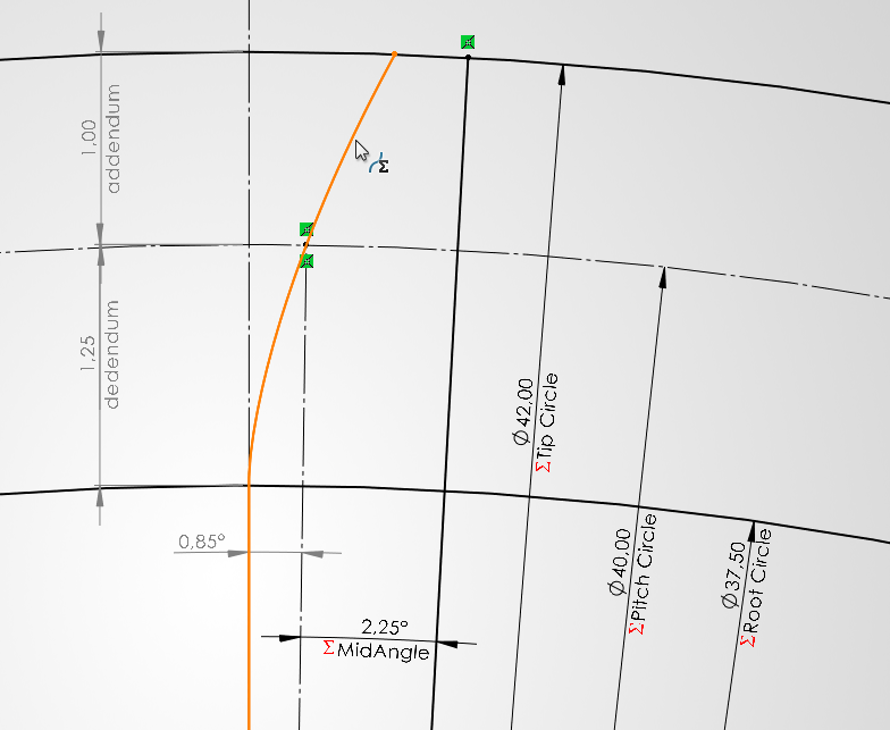
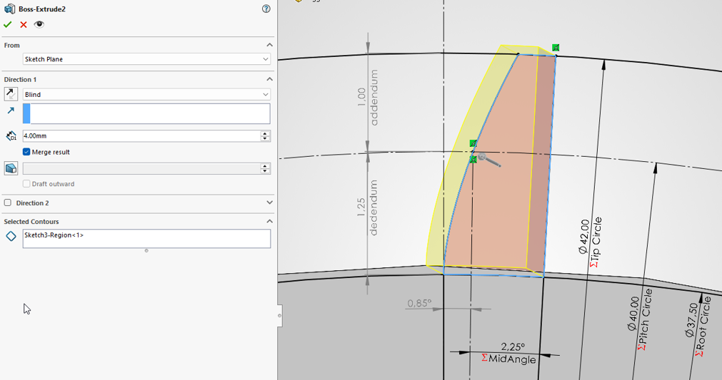
MidAngle \(= 2.25°\) from there to the tooth centreline.
Selecting contours instead of trimming
The flank deliberately overshoots, reaching down to \(r_b(1 - t_\text{tip})\), which is \(3.68\) mm at \(N = 20\) against a root radius of \(8.75\) mm. It has to overshoot, because \(t_1\) is set once and must place the start of the curve below the root circle for every tooth count we care about.
We do not trim the overshoot away, because we cannot. SolidWorks refuses to shorten an equation driven curve, and Mirror Entities likewise either refuses or converts the curve to an ordinary spline and severs its link to the global variables. Attempting either is how this construction is usually broken.
Instead we let the overshoot stand and choose contours. Where the overshoot crosses the root arc it divides the sketch into several closed regions, and the extrusion takes only the one we want. Use Selected Contours and pick the half tooth. Whatever regions the overshoot cuts off below the root arc are simply left unselected, and their number may change with \(N\) without affecting anything. Figure 9.2.5 shows the single entry this leaves in the Selected Contours field.
Extruding, patterning and mirroring
Sketch a circle of radius RootRadius on the Top Plane and extrude it Blind by "FaceWidth". This is the gear body up to the root. Then extrude the half tooth sketch, also Blind by "FaceWidth", using the contour from the previous section and leaving Merge result on so the tooth fuses to the body.
Both choices are deliberate. The sketch sits on a datum plane rather than on a model face, and the end condition is Blind rather than any of the up to conditions, because a circular pattern re-creates each instance from the feature definition rather than copying solid geometry. Every reference the seed carries has to still resolve after the feature has been rotated, and a reference to a particular face does not.
Add the root fillet next, as a feature rather than in the sketch, and add it before the pattern rather than after. Fillet the root edge where the tooth flank meets the root cylinder, radius "R_fillet", with tangent propagation on, as in Figure 9.2.6. Filleting now means one edge is blended and then copied \(N\) times; filleting after the pattern means selecting \(2N\) edges. SolidWorks solves the tangency itself, which matters because above roughly \(N = 25\) that tangency point is no longer on the straight part of the flank.
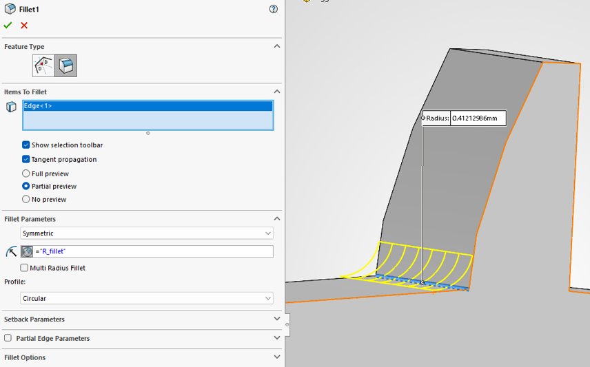
= "R_fillet" rather than a number, so the fillet tracks the tooth count, and Tangent propagation carries the blend along the root edge. Letting SolidWorks solve the tangency is what allows the same construction to work once that point migrates from the radial segment onto the involute.
Add a reference axis through the gear centre from Insert, Reference Geometry, Axis, selecting the Front Plane and the Right Plane. Their intersection is the gear axis, defined by datums alone. Do not use a model edge or face for this: both are topological indices that renumber on rebuild.
Circular pattern the tooth together with its fillet about that axis, equal spacing over \(360°\), and tie the count to the profile by adding
"D1@CirPattern1" = "N"to the equations. Leave Geometry pattern unchecked. Figure 9.2.7 shows the completed dialog.
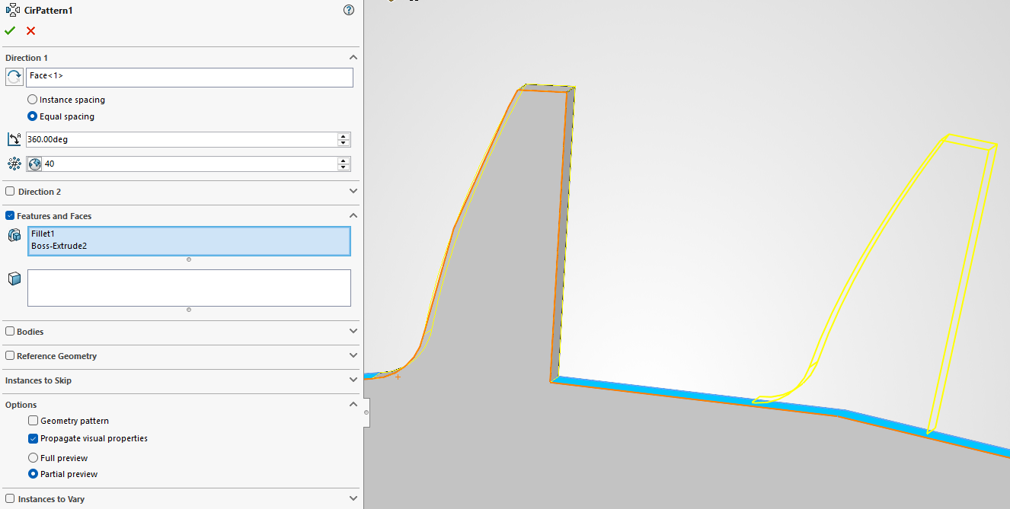
Fillet1 and Boss-Extrude2 in the features box and the faces box left empty. Direction 1 here holds Face<1>. A cylindrical face does supply a valid axis, but it is a topological reference, and the datum axis described above is what survives a large change in \(N\).
Mirror last. Build the mirror plane from datums: Insert, Reference Geometry, Plane, taking the Right Plane at angle "MirrorAngle" about the gear axis, with MirrorAngle as given under why the datum must be the pitch circle. Do not pick a model face. A face is a topological index, and a large change in \(N\) regenerates the solid, loses the reference and fails the mirror with Could not find face or plane. A plane built from the Right Plane, the axis and an equation has nothing to lose. Figure 9.2.8 shows the field in question.
Then mirror the tooth extrusion and its fillet together with the circular pattern. The pattern feature holds only the copies, not the seed, so mirroring the pattern alone leaves one tooth with half a profile. Leave the root cylinder out of the mirror, since it is already symmetric about every plane through the axis and including it only produces a coincident duplicate.
The ordering is not a matter of taste. A mirror feature carries its mirror plane as a reference, and when that plane is a model face it cannot be reconstructed at the rotated positions, so patterning the mirror fails. Checking Geometry pattern would skip the re-solve, but SolidWorks declines to apply it to a mirror seed. Building the plane from datums removes that particular failure; placing the mirror after the pattern avoids the question entirely, which is what we do here.
Mirroring the whole array rather than the single tooth is exact, not an approximation. A reflection conjugates a rotation into its inverse, so the mirror of half tooth \(k\) lands on the missing half of tooth \(-k\), and letting \(k\) run over all \(N\) covers every remaining half.
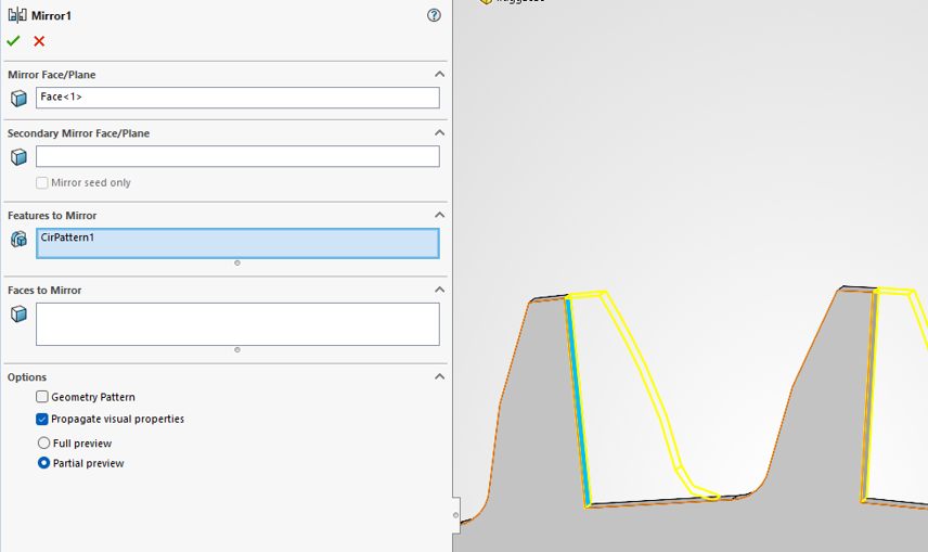
CirPattern1; the seed features have to go in alongside it, or the tooth the pattern grew from keeps only half its profile. The Mirror Face/Plane field here holds Face<1>, which is the reference that fails on a large change of \(N\); it should be the datum plane described above.
Checking the model
Set N to \(12\), rebuild, then to \(50\), and rebuild again. These straddle the crossover of 9.2.1, so a model that survives both has exercised the straight portion of the flank and the case where it is not used. Then measure the tooth thickness along the pitch circle: at \(m = 1\) it must be \(\pi m/2 = 1.5708\) mm. A gear that looks right but measures short is the symptom described under why the datum must be the pitch circle.
Robustness and its limits
Within the range this construction is meant for, the sketch contains the same entities for every \(N\): one equation driven curve, two arcs and one line. The curve is continuous from below the root to the tip, the root edge the fillet blends always exists, and the parameter bounds never move off \(t \in [-1, 1]\). Nothing in the sketch depends on whether \(r_f\) is larger or smaller than \(r_b\), which is the discontinuity that usually forces a rebuild failure.
The construction does have limits, and they are set by the tooth proportions rather than by the modelling. Below about \(18\) teeth a gear generated by a rack undercuts, the cutter removing part of the flank near the base circle, and the model built here does not reproduce that. It draws the full involute down to the root regardless, so for small \(N\) it describes a gear that a hob would not actually cut. At the other end \(R_\text{fillet}\) shrinks as \(N\) grows, falling below one \(0.4\) mm extrusion width at about \(N = 42\) and passing through zero at \(N = 105\). The model itself has been rebuilt successfully from \(N = 8\) to \(N = 100\), so buildability is not what limits it. Usefulness is: outside roughly \(18\) to \(60\) teeth the part either is not the gear a hob would cut or has a root fillet too small to print. Both bounds are worked out under the root fillet radius and limits of the model.
Derivations
The rest of the chapter justifies the expressions used above. None of it is needed to build the gear.
Why the datum must be the pitch circle
Tooth thickness is defined at the pitch circle, where standard proportions divide the circular pitch equally between tooth and space, giving \(t_p = \pi m / 2\). Carried to any other radius along the involute, the thickness becomes
\[ t_r = 2r\left(\frac{t_p}{2 r_p} + \operatorname{inv}\varphi - \operatorname{inv}\varphi_r\right) \tag{9.2.6}\]
where \(\varphi_r\) is the pressure angle at radius \(r\) [3,4]. Setting \(r = r_b\) makes \(\varphi_b = 0\), so \(\operatorname{inv}\varphi_b = 0\) and the bracket loses the term that distinguished one radius from another. The base circle carries no thickness information.
This is why the datum line of the sketch procedure runs to the pitch circle. Referencing it instead to the point where the involute leaves the base circle is the tempting mistake, since that point is where the curve visibly starts and is trivial to snap to, but it is the one radius where the construction degenerates. Doing so drops \(\operatorname{inv}\varphi\) from the half tooth angle, and every tooth comes out \(2\operatorname{inv}\varphi = 1.71°\) too thin. At \(N = 20\) and \(m = 1\) that is a pitch circle thickness of \(1.273\) mm against the correct \(1.571\) mm, an error of \(19\%\) which is not visible by eye but which no gear will mesh with. This correction is due to Mick of Kusel Design, Australia, who identified it in an earlier version of this construction.
Equivalently, the construction line can be dispensed with and the mirror line dimensioned straight from the cusp line through
\[ \psi_c = \frac{\pi}{2N} + \operatorname{inv}\varphi \tag{9.2.7}\]
which in the equation manager reads
"MirrorAngle" = 90 / "N" + (tan("PressureAngle") - "PressureAngle" * pi / 180) * 180 / piand evaluates to \(5.354°\) at \(N = 20\). The two constructions give the same tooth. The first makes the geometry visible in the sketch, the second removes an entity.
Replacing a conditional with algebra
For any real \(v\), \(\sqrt{v^2} = |v|\), and therefore
\[ \max(v, 0) = \frac{v + \sqrt{v^2}}{2}, \qquad \min(v, 0) = \frac{v - \sqrt{v^2}}{2} \tag{9.2.8}\]
Each expression returns \(v\) when \(v\) has the matching sign and zero otherwise, using nothing but arithmetic and a square root. In SolidWorks syntax these are (v + sqr(v ^ 2)) / 2 and (v - sqr(v ^ 2)) / 2, which is where the repetition in the curve expressions of the flank comes from.
The identity earns its place because the alternative is worse. The equation driven curve dialog provides arithmetic, powers and the elementary functions, and no conditional of any kind. Without 9.2.8 the flank would have to be drawn as two entities, a line below the base circle and an involute above it, and the line would then have to disappear when \(r_f > r_b\). The sketch topology would depend on \(N\), and at the crossover of 9.2.1 every relation and fillet attached to the vanishing line would break. Writing the branch algebraically buys a fixed topology, which is the whole point of the exercise.
The root fillet radius
The fillet used here is not a standard one. A hobbed gear gets its root fillet from the tip radius of the generating rack, which ISO 53 sets at \(\rho_{fP} = 0.38\,m\) for the standard basic rack tooth profile, its informative annex offering \(0.30\,m\), \(0.25\,m\) and \(0.39\,m\) as alternatives for lighter loading and for full root radius work [1]. Reproducing that fillet means simulating the cutter, which we are not doing.
The standard value is worth a second look, because it is not an arbitrary choice either. For a \(20°\) rack with bottom clearance \(c_P < 0.295\,m\), ISO 53 gives the largest fillet the clearance admits as
\[ \rho_{fP\max} = \frac{c_P}{1 - \sin\alpha_P} \]
and the standard clearance \(c_P = 0.25\,m\) returns \(0.3800\,m\), which is the tabulated \(0.38\,m\). The standard fillet is therefore the largest one that fits, quoted to two figures. We apply the same principle to the gear rather than to the rack: take the largest arc that fits the tooth space, then back away from it.
Subtracting the tooth thickness of 9.2.6 from the circular pitch at the base circle leaves a space whose half width is
\[ \frac{e_b}{2} = r_b\left(\frac{\pi}{2N} - \operatorname{inv}\varphi\right) \tag{9.2.9}\]
and we take \(R_f = 0.9\,e_b/2\), which is the expression in the table of global variables.
The factor \(0.9\) deserves more scrutiny than it usually gets, because the fillet does not sit at the base circle. It sits at the root, where the space is narrower. Two fillets from adjacent teeth clear one another when the arc each subtends on the root circle is smaller than the half space there,
\[ \arcsin\frac{R_f}{r_f + R_f} < \beta, \qquad \beta = \frac{\pi}{2N} - \operatorname{inv}\varphi \tag{9.2.10}\]
or equivalently \(R_f < r_f \sin\beta / (1 - \sin\beta)\). The bound of 9.2.10 permits \(0.594\) mm at \(N = 20\) against the \(0.538\) mm we use, a margin of \(9\%\). Across the usable range the ratio of the fillet we take to the largest that fits runs from \(0.87\) at large \(N\) to \(0.97\) at \(N = 10\), so the nominal \(0.9\) is not the safety factor it appears to be, and it is tightest exactly where teeth are fewest. At \(N = 8\) it crosses over: \(R_f = 0.614\) mm against a limit of \(0.606\) mm, so the two fillets in one space just overlap. Made as a feature this is harmless and arguably an improvement, because the two blends merge into a single continuous rounded root, which is what ISO 53 calls a full root radius profile. Made in the sketch it would have been an error.
Two further consequences decide how the fillet has to be built. Above about \(N = 25\) the tangency point leaves the straight part of the flank and lands on the involute, because \(\sqrt{r_f^2 + 2 r_f R_f}\) then exceeds \(r_b\). A sketch fillet has to be told where that point is and a fillet feature on the root edge simply solves for it, which is why the guide fillets the solid rather than the sketch.
At the other end the fillet quietly disappears. 9.2.9 shrinks with \(N\), giving \(R_f = 0.16\) mm at \(N = 80\) and \(0.034\) mm at \(N = 100\), before turning negative when \(\pi/(2N) = \operatorname{inv}\varphi\), that is at \(N = 105\). A \(0.034\) mm fillet laid down by a \(0.4\) mm nozzle does not exist. The feature still reports success, so from about \(N = 42\) upwards the model rebuilds and the part has a fillet stop being the same statement.
Limits of the model
A rack cutter generating a gear of few teeth removes material below the base circle that the involute would otherwise occupy. The flank is then undercut, and the tooth is both weaker and shorter in its usable profile. The condition for a rack generated gear to avoid undercut without profile shift is \(N \geq 2/\sin^2\varphi\), which is \(17.1\) and therefore \(18\) teeth at \(20°\) [4]. Our model has no cutter and draws the full involute regardless, so below \(18\) teeth it produces a geometrically valid involute gear that is not the gear a hob would cut.
The usual remedy is profile shift, moving the cutter radially so that the tooth is generated further out along the involute. This changes the pitch circle thickness to \(t_p = m(\pi/2 + 2x\tan\varphi)\) for a shift \(x\), so MidAngle is then no longer a quarter of the angular pitch and 9.2.7 acquires an extra term. Nothing else in the construction changes. The model as given assumes \(x = 0\) throughout.
Two further simplifications are worth stating. No backlash allowance is included, so a pair of these gears meshes with zero theoretical clearance and a real pair would need the tooth thickness reduced slightly. No tip relief is included either, so the profile runs sharp to the tip circle where a loaded gear would normally have the corner eased.
References
[1]
ISO 53:1998 Cylindrical gears for general and heavy engineering – Standard basic rack tooth profile. Geneva, Switzerland: International Organization for Standardization; 1998.
[2]
Litvin FL, Fuentes A. Gear geometry and applied theory. 2nd ed. Cambridge: Cambridge University Press; 2004.
[3]
Buckingham E. Analytical mechanics of gears. New York: Dover Publications; 1988.
[4]
Budynas RG, Nisbett JK. Shigley’s mechanical engineering design. 11th ed. New York: McGraw-Hill Education; 2020.