8.8  Hooke’s law in 3D

Superposition of uniaxial responses

Start from what we know. A uniaxial stress \(\sigma_x\) produces a strain \(\sigma_x/E\) along its own direction, and by 8.6.4 it also produces a contraction \(-\nu\sigma_x/E\) in each of the two transverse directions. For small strains the response is linear, so the strains produced by three simultaneous normal stresses simply add. The strain along \(x\) is its own direct response plus the transverse contributions of the other two,

\[ \left.\begin{array}{l} \varepsilon_x = \dfrac{\sigma_x}{E} - \nu\left(\dfrac{\sigma_y}{E} + \dfrac{\sigma_z}{E}\right)\\[8pt] \varepsilon_y = \dfrac{\sigma_y}{E} - \nu\left(\dfrac{\sigma_x}{E} + \dfrac{\sigma_z}{E}\right)\\[8pt] \varepsilon_z = \dfrac{\sigma_z}{E} - \nu\left(\dfrac{\sigma_x}{E} + \dfrac{\sigma_y}{E}\right) \end{array}\right\} \qquad \begin{bmatrix}\varepsilon_x\\ \varepsilon_y\\ \varepsilon_z\end{bmatrix} = \frac{1}{E}\begin{bmatrix} 1 & -\nu & -\nu\\ -\nu & 1 & -\nu\\ -\nu & -\nu & 1 \end{bmatrix} \begin{bmatrix}\sigma_x\\ \sigma_y\\ \sigma_z\end{bmatrix} \tag{8.8.1}\]

The matrix in 8.8.1 is the compliance: it turns stress into strain. For design we usually want the opposite direction, so we invert it.

E, nu = sp.symbols('E nu', positive=True)

compliance = sp.Matrix([[1, -nu, -nu],
                        [-nu, 1, -nu],
                        [-nu, -nu, 1]]) / E

stiffness = sp.simplify(compliance.inv())
ltx(r"\bm C^{-1} =", sp.factor(stiffness))

Reading off the first row and grouping the terms so that the sum of the normal strains appears as a unit, the inverted relation is

\[ \begin{array}{l} \sigma_x = \dfrac{E}{1+\nu}\left(\varepsilon_x + \dfrac{\nu}{1-2\nu}\left(\varepsilon_x + \varepsilon_y + \varepsilon_z\right)\right)\\[10pt] \sigma_y = \dfrac{E}{1+\nu}\left(\varepsilon_y + \dfrac{\nu}{1-2\nu}\left(\varepsilon_x + \varepsilon_y + \varepsilon_z\right)\right)\\[10pt] \sigma_z = \dfrac{E}{1+\nu}\left(\varepsilon_z + \dfrac{\nu}{1-2\nu}\left(\varepsilon_x + \varepsilon_y + \varepsilon_z\right)\right) \end{array} \tag{8.8.2}\]

Note the factor \(1-2\nu\) in the denominator. It vanishes at \(\nu = 1/2\), and 8.8.3 below shows what that means physically.

The bulk modulus

The bulk modulus \(K\) measures resistance to a change of volume. Define the mean stress \(\sigma_m\) and the volumetric strain \(\Delta\) as

\[ \sigma_m = \frac{\sigma_x + \sigma_y + \sigma_z}{3}, \qquad \Delta = \varepsilon_x + \varepsilon_y + \varepsilon_z \]

and \(K := \sigma_m/\Delta\). Adding the three rows of 8.8.1 gives the volumetric strain in terms of the stresses,

\[ \Delta = \frac{1-2\nu}{E}\left(\sigma_x + \sigma_y + \sigma_z\right) = \frac{3(1-2\nu)}{E}\,\sigma_m \]

so that the bulk modulus is

\[ \boxed{K = \frac{\sigma_m}{\Delta} = \frac{E}{3(1-2\nu)}} \tag{8.8.3}\]

which grows without bound as \(\nu \to 1/2\). A material with \(\nu = 1/2\) cannot have its volume changed by any finite pressure: it is incompressible. Rubber, with \(\nu = 0.4999\), is close enough that finite element codes need special elements to handle it, because the stiffness matrix becomes ill-conditioned as the volumetric term dominates everything else.

The shear modulus

We asserted in 8.5.8 that the shear modulus is not independent of \(E\) and \(\nu\). The proof uses the principal stress machinery of the previous chapter.

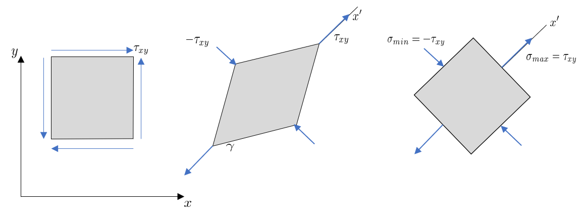
Consider an element in pure shear, Figure 8.8.1, with \(\sigma_x = \sigma_y = 0\) and a shear stress \(\tau_{xy}\). Its principal stresses follow from 8.7.11 as \(\sigma_1 = \tau_{xy}\) and \(\sigma_2 = -\tau_{xy}\), with \(\sigma_3 = 0\) out of the plane: pure shear is the same state as equal tension and compression at \(45^\circ\).

Substituting these three principal stresses into the first row of 8.8.1 gives the largest principal strain

\[ \varepsilon_1 = \frac{\sigma_1}{E} - \nu\left(\frac{\sigma_2}{E} + \frac{\sigma_3}{E}\right) = \frac{\tau_{xy}}{E} - \nu\left(\frac{-\tau_{xy}}{E} + 0\right) = \frac{\tau_{xy}}{E}\left(1+\nu\right) \tag{8.8.4}\]

The same state expressed in the original frame has \(\varepsilon_x = \varepsilon_y = 0\) and shear strain \(\gamma_{xy}\), so 8.7.12 gives the largest principal strain as

\[ \varepsilon_1 = \frac{\gamma_{xy}}{2} \]

Equating the two expressions for \(\varepsilon_1\) and using \(\tau_{xy} = G\gamma_{xy}\) from 8.5.7 gives

\[ \frac{\gamma_{xy}}{2} = \frac{\tau_{xy}(1+\nu)}{E} = \frac{G\gamma_{xy}(1+\nu)}{E} \quad\Longrightarrow\quad \boxed{G = \frac{E}{2(1+\nu)}} \tag{8.8.5}\]

which completes the proof. An isotropic material has exactly two independent elastic constants, and \(E\), \(\nu\), \(G\) and \(K\) are four different ways of naming pairs of them.

Generalized Hooke’s law

We can now write the constitutive relation in tensor form. The shear components follow from 8.8.5 combined with the tensor shear strain \(\varepsilon_{xy} = \tfrac{1}{2}\gamma_{xy}\),

\[ \tau_{xy} = G\gamma_{xy} = 2G\varepsilon_{xy} = \frac{E}{1+\nu}\varepsilon_{xy} \]

and the normal components follow from expanding 8.8.2,

\[ \sigma_x = \underbrace{\frac{E}{1+\nu}}_{2\mu\,=\,2G}\varepsilon_x + \underbrace{\frac{E\nu}{(1+\nu)(1-2\nu)}}_{\lambda}\left(\varepsilon_x + \varepsilon_y + \varepsilon_z\right) \]

Both terms carry the same two constants, which we name the Lamé parameters

\[ \boxed{\mu = G = \frac{E}{2(1+\nu)}, \qquad \lambda = \frac{E\nu}{(1+\nu)(1-2\nu)}} \tag{8.8.6}\]

With these, all six components collapse into a single matrix equation,

\[ \begin{bmatrix} \sigma_x & \tau_{xy} & \tau_{xz}\\ \tau_{xy} & \sigma_y & \tau_{yz}\\ \tau_{xz} & \tau_{yz} & \sigma_z \end{bmatrix} = 2\mu \begin{bmatrix} \varepsilon_x & \varepsilon_{xy} & \varepsilon_{xz}\\ \varepsilon_{xy} & \varepsilon_y & \varepsilon_{yz}\\ \varepsilon_{xz} & \varepsilon_{yz} & \varepsilon_z \end{bmatrix} + \lambda \underbrace{\begin{bmatrix}1&0&0\\0&1&0\\0&0&1\end{bmatrix}}_{\bm I} \underbrace{\left(\varepsilon_x + \varepsilon_y + \varepsilon_z\right)}_{\operatorname{tr}\bm\varepsilon \,=\, \nabla\cdot\bm u} \]

which is the generalized Hooke’s law for isotropic materials

\[ \boxed{\bm\sigma = 2\mu\,\bm\varepsilon + \lambda \operatorname{tr}(\bm\varepsilon)\,\bm I} \qquad\text{or}\qquad \bm\sigma = 2\mu\,\bm\varepsilon + \lambda \left(\nabla\cdot\bm u\right)\bm I \tag{8.8.7}\]

A quick check of two entries confirms the reading: \(\sigma_y = 2\mu\varepsilon_y + \lambda\operatorname{tr}\bm\varepsilon\) and \(\tau_{xz} = 2\mu\varepsilon_{xz}\), as they should be. The two terms have distinct physical meanings. The first is proportional to the strain itself and represents distortion, the change of shape. The second is proportional to the identity and to the volume change, and represents dilatation. The same split applied to the stress gives the deviatoric and volumetric stress tensors, and it is the deviatoric part alone that drives yielding through 8.7.13.

The relation inverts to

\[ \bm\varepsilon = \frac{1}{2\mu}\bm\sigma - \frac{\lambda}{2\mu(3\lambda + 2\mu)}\operatorname{tr}(\bm\sigma)\,\bm I \tag{8.8.8}\]

which we verify symbolically rather than by hand.

mu_s, lam_s = sp.symbols('mu lambda', positive=True)

Sigma = sp.Matrix(3, 3, lambda i, j: sp.Symbol(f'sigma_{min(i,j)}{max(i,j)}'))
Eps = Sigma/(2*mu_s) - lam_s/(2*mu_s*(3*lam_s + 2*mu_s))*sp.trace(Sigma)*sp.eye(3)
recovered = sp.simplify(2*mu_s*Eps + lam_s*sp.trace(Eps)*sp.eye(3))

ltx(r"2\mu\bm\varepsilon + \lambda\,\mathrm{tr}(\bm\varepsilon)\bm I - \bm\sigma =",
    sp.simplify(recovered - Sigma))

The residual is the zero matrix, so 8.8.8 is the exact inverse of 8.8.7.

Volumetric strain and incompressibility

Consider a cube of side \(a\) strained by \(\varepsilon_x\), \(\varepsilon_y\) and \(\varepsilon_z\). Its deformed volume is the product of the three stretched sides,

\[ V = a^3(1+\varepsilon_x)(1+\varepsilon_y)(1+\varepsilon_z) \approx a^3\left(1 + \varepsilon_x + \varepsilon_y + \varepsilon_z\right) \]

where the products of strains have been dropped as second order. The relative change of volume is therefore

\[ \frac{\Delta V}{V_0} = \varepsilon_x + \varepsilon_y + \varepsilon_z = \operatorname{tr}\bm\varepsilon =: I_1 \tag{8.8.9}\]

the trace of the strain tensor, also called the first invariant because it is unchanged by rotation of the frame.

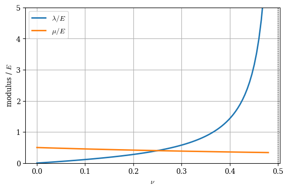
Now return to the Lamé parameter \(\lambda = E\nu/((1+\nu)(1-2\nu))\) and let \(\nu\) approach \(1/2\). The parameter grows without bound, and since \(\lambda\) multiplies \(\operatorname{tr}\bm\varepsilon\) in 8.8.7, the only way for the stress to stay finite is for the trace to go to zero. An infinite \(\lambda\) therefore forces \(\Delta V/V_0 \to 0\): the material becomes incompressible. Plotting the two Lamé parameters against Poisson’s ratio shows how differently they behave.

E_val = 210e3

lam_expr = E*nu/((1+nu)*(1-2*nu))
mu_expr = E/(2*(1+nu))

fig, ax = plt.subplots(figsize=(6.5, 4))
fplot(lam_expr.subs(E, E_val)/E_val, (nu, 0, 0.48), ax=ax, linewidth=2,
      label=r"$\lambda / E$")
fplot(mu_expr.subs(E, E_val)/E_val, (nu, 0, 0.48), ax=ax, linewidth=2,
      label=r"$\mu / E$")
ax.axvline(0.5, color='k', linestyle=':', linewidth=1)
ax.set_xlabel(r"$\nu$")
ax.set_ylabel("modulus / $E$")
ax.set_ylim(0, 5)
ax.grid(True)
ax.legend()
plt.show()

The shear modulus falls gently from \(E/2\) to \(E/3\) over the whole physical range, while \(\lambda\) is nearly flat up to \(\nu \approx 0.3\) and then runs away. Steel at \(\nu = 0.3\) sits at the start of the steep part, rubber at \(0.4999\) is far up it, and cork at \(\nu = 0\) has \(\lambda = 0\) and no coupling between directions at all.

Two-dimensional simplifications

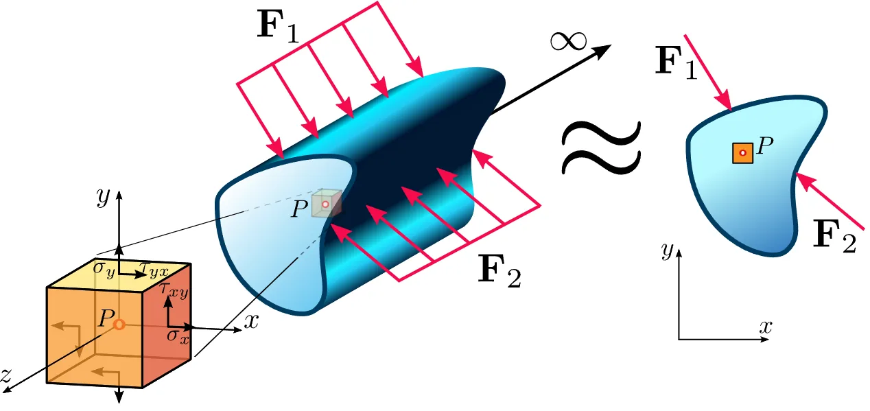
Solving 8.7.7 together with 8.8.7 in three dimensions is expensive, and a large fraction of engineering geometry is close enough to one of two special cases that the third dimension can be eliminated in advance. Both cases keep the same physics and reduce the problem to two dimensions, which cuts the size of a finite element model by orders of magnitude.

Plane strain

Plane strain applies when the structure is much longer in one direction than in the other two and is loaded uniformly along its length: a dam, a tunnel lining, a long pipe, a gear tooth taken out of a wide gear. Material far from the ends cannot move along the length because the material either side of it is doing the same thing, so all strain components involving \(z\) vanish and the strain tensor becomes

\[ \bm\varepsilon = \begin{bmatrix} \varepsilon_x & \varepsilon_{xy} & 0\\ \varepsilon_{xy} & \varepsilon_y & 0\\ 0 & 0 & 0 \end{bmatrix} \]

Zero strain in \(z\) does not mean zero stress in \(z\). Substituting \(\varepsilon_z = 0\) into 8.8.2 leaves

\[ \sigma_z = \frac{E}{1+\nu}\left(0 + \frac{\nu}{1-2\nu}\left(\underbrace{\varepsilon_x + \varepsilon_y}_{\neq 0}\right)\right) = \lambda\left(\varepsilon_x + \varepsilon_y\right) \]

so the stress tensor keeps a non-zero \(zz\) component,

\[ \bm\sigma = \begin{bmatrix} \sigma_x & \tau_{xy} & 0\\ \tau_{xy} & \sigma_y & 0\\ 0 & 0 & \sigma_z \end{bmatrix} \]

which is exactly the constraint stress required to hold the material in place along its length. The in-plane part of Hooke’s law keeps its three-dimensional form with the trace taken over the two remaining directions,

\[ \begin{bmatrix}\sigma_x & \tau_{xy}\\ \tau_{xy} & \sigma_y\end{bmatrix} = \frac{E}{1+\nu}\left( \begin{bmatrix}\varepsilon_x & \varepsilon_{xy}\\ \varepsilon_{xy} & \varepsilon_y\end{bmatrix} + \frac{\nu}{1-2\nu}\begin{bmatrix}1&0\\0&1\end{bmatrix}\left(\varepsilon_x + \varepsilon_y\right)\right) \tag{8.8.10}\]

so the Lamé parameters of 8.8.6 carry over unchanged.

Plane stress

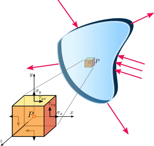
Plane stress applies to the opposite geometry: a thin sheet loaded in its own plane, with nothing pressing on the free faces. A plate with a hole, a bracket cut from sheet metal, a thin-walled pressure vessel or a laser-cut chassis panel all qualify. There is no material above or below to carry stress through the thickness, so

\[ \bm\sigma = \begin{bmatrix} \sigma_x & \tau_{xy} & 0\\ \tau_{xy} & \sigma_y & 0\\ 0 & 0 & 0 \end{bmatrix} \]

The roles are now reversed. The stress through the thickness is zero but the strain is not: setting \(\sigma_z = 0\) in 8.8.1 gives

\[ \varepsilon_z = -\nu\left(\frac{\sigma_x}{E} + \frac{\sigma_y}{E}\right) \tag{8.8.11}\]

so the sheet gets thinner as it is stretched, which is Poisson’s effect and is entirely expected. Eliminating \(\varepsilon_z\) from 8.8.7 leaves the in-plane relation

\[ \begin{bmatrix}\sigma_x & \tau_{xy}\\ \tau_{xy} & \sigma_y\end{bmatrix} = \frac{E}{1-\nu^2}\left( (1-\nu)\begin{bmatrix}\varepsilon_x & \varepsilon_{xy}\\ \varepsilon_{xy} & \varepsilon_y\end{bmatrix} + \nu\begin{bmatrix}1&0\\0&1\end{bmatrix}\left(\varepsilon_x + \varepsilon_y\right)\right) \tag{8.8.12}\]

which has the same shape as 8.8.10 but with a modified first Lamé parameter,

\[ \lambda^* = \frac{2\mu\lambda}{\lambda + 2\mu} = \frac{E\nu}{1-\nu^2}, \qquad \mu^* = \mu = \frac{E}{2(1+\nu)} \tag{8.8.13}\]

The shear modulus is untouched, since shearing in the plane does not involve the thickness at all. Let us confirm the substitution symbolically.

Code

lam_3d = E*nu/((1+nu)*(1-2*nu))
mu_3d = E/(2*(1+nu))

lam_star = sp.simplify(2*mu_3d*lam_3d/(lam_3d + 2*mu_3d))

ltx(r"\lambda^* &=", lam_star,
    r"\\ \frac{E\nu}{1-\nu^2} - \lambda^* &=",
    sp.simplify(E*nu/(1-nu**2) - lam_star), aligned=True)

\[ \begin{aligned}\lambda^* &=\dfrac{E \nu}{1 - \nu^{2}}\\ \frac{E\nu}{1-\nu^2} - \lambda^* &=0\end{aligned} \]

Choosing between the two models is a modelling decision with real consequences, and choosing wrongly produces stresses that are wrong by a factor of order \(1/(1-\nu^2)\). The test is whether the material through the thickness is constrained or free. Constrained means plane strain, free means plane stress. A gear tooth in the middle of a wide gear is constrained; the same tooth on a thin sprocket is free.

Example: A plate in biaxial tension

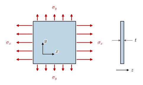
A thin steel plate, \(E = 210\,000~\text{MPa}\) and \(\nu = 0.3\), is loaded in its plane to \(\sigma_x = 150~\text{MPa}\) and \(\sigma_y = 60~\text{MPa}\) with no shear. Determine the three normal strains, the change in thickness of a \(2~\text{mm}\) plate, and the volumetric strain.

E_v, nu_v = 210e3, 0.3
sig = sp.Matrix([150, 60, 0])                      # plane stress

C = sp.Matrix([[1, -nu_v, -nu_v],
               [-nu_v, 1, -nu_v],
               [-nu_v, -nu_v, 1]]) / E_v

eps = C * sig
t0 = 2.0                                            # plate thickness [mm]

ltx(r"\varepsilon_x &=", eps[0], r"\\ \varepsilon_y &=", eps[1],
    r"\\ \varepsilon_z &=", eps[2],
    r"\\ \Delta t &=", t0*eps[2], r"~\text{mm}",
    r"\\ \mathrm{tr}\,\bm\varepsilon &=", sum(eps), aligned=True, precision=3)

The plate stretches in both loaded directions and thins by \(6\times10^{-4}~\text{mm}\), which is \(0.6~\mu\text{m}\) on a \(2~\text{mm}\) plate. The volumetric strain is positive: the plate gains volume under biaxial tension, as 8.8.9 requires whenever the mean stress is positive.

A common mistake is to assume that zero stress through the thickness means the plate keeps its thickness. 8.8.11 says otherwise, and the distinction matters in sheet forming, where thinning is the failure mode that limits how far a panel can be drawn.

Closing the continuum model

The model is now complete. Kinematics relates displacement to strain through 8.7.3, the constitutive law relates strain to stress through 8.8.7, and equilibrium relates stress to the applied load through 8.7.7 and 8.7.8. Chaining the three together gives one vector equation for the displacement field,

\[ -\nabla \cdot \left(2\mu\,\bm\varepsilon(\bm u) + \lambda\left(\nabla\cdot\bm u\right)\bm I\right) = \bm f \tag{8.8.14}\]

known as the Navier equation, which together with boundary conditions determines everything about a linearly elastic body. Solving it in general requires the finite element method. Solving it for special geometries by hand is what classical solid mechanics does, and each classical theory is 8.8.14 plus an assumption about how the displacement field varies over a cross section. The beam theory of Chapter 8.14 is the most useful of them.