8.6 Material properties and the tensile test
“Was man mit Fehlerrechnung nicht beschreiben kann, darüber muss man schweigen.”
“Whereof one cannot state an uncertainty, thereof one must be silent.”
— after Ludwig Wittgenstein, Tractatus Logico-Philosophicus, 1921, proposition 7, as physicists retell it
We now have a measure of internal force and a measure of deformation, and they are logically independent: nothing said so far connects them. The connection is supplied by the material, through a constitutive relation, and unlike equilibrium and kinematics it cannot be derived. It has to be measured. This chapter covers the simplest such relation, linear elasticity, the experiment that produces it, and what to do when the material in front of you does not obey it.
That last part carries most of the weight. Linear elasticity describes a material that is linear and isotropic, and the specimens in this chapter are neither.
They are made by fused filament fabrication, or FFF, which is what an ordinary desktop 3D printer does: a thermoplastic filament is melted and laid down as a sequence of adjacent roads, stacked in layers, each fusing to its neighbours as it cools. The material is polylactic acid, PLA, a stiff thermoplastic polyester that is the usual filament on such machines and the one the laboratory uses. A printed part is therefore not a block of PLA. It is an assembly of PLA roads together with the bonds between them, and that distinction runs through everything below.
Metals fit this theory far better, and they are not absent here. The idealised curve below is a ductile metal, the offset yield convention comes from the metals standards, and the moduli tabulated in the next section are for steel, aluminium and titanium, because that is where linear elasticity is most convincing and where its whole vocabulary was invented.
The measurements are printed PLA for two reasons. It is the material our students actually manufacture with, so it is the one whose stiffness they will need to know. And a material that fits the model exactly teaches nothing about the model: evaluate a mild steel bar and linear elasticity looks like a fact about nature, whereas evaluating something that resists the assumptions makes the edges of the model visible, and that is the more useful thing to come away with. Why printing runs through the book at all is set out in the introduction.
We fit the linear model anyway, because no part can be sized without a stiffness, but fitting it is a modelling decision with conditions attached and not the measurement of a constant. Keeping those two things apart is the whole subject of this chapter.
Hooke’s law and Young’s modulus
The simplest constitutive relation is linear,
\[ \boxed{\sigma = E\varepsilon} \tag{8.6.1}\]
known as Hooke’s law, in which the constant of proportionality \(E\) is the Young’s modulus, or modulus of elasticity. It has the same units as stress, since strain is dimensionless, and it is the stiffness of the material in the same way that a spring constant is the stiffness of a spring.
Code
from scipy.interpolate import PchipInterpolator

# Anchor points for a schematic ductile response. Not to scale.
e_pl, s_pl = 0.13, 0.55          # proportional limit
e_el, s_el = 0.16, 0.60          # elastic limit
e_Y,  s_Y  = 0.22, 0.62          # yield stress, start of the plateau
e_p2       = 0.55                # end of the yield plateau
e_u,  s_u  = 1.40, 1.00          # ultimate stress
e_f,  s_f  = 2.00, 0.80          # fracture, engineering
s_tf       = 1.62                # true fracture stress

eng = PchipInterpolator([0, e_pl, e_el, e_Y, e_p2, 0.80, 1.05, e_u, 1.70, e_f],
                        [0, s_pl, s_el, s_Y, s_Y,  0.82, 0.93, s_u, 0.97, s_f])
tru = PchipInterpolator([0, e_pl, e_Y, e_p2, 0.80, 1.05, e_u, 1.70, e_f],
                        [0, s_pl, s_Y, 0.70, 0.90, 1.02, 1.16, 1.36, s_tf])
x = np.linspace(0, e_f, 700)

fig, ax = plt.subplots(figsize=(8.4, 5.8))
CURVE = '#1F7A99'

for x0, x1, colour, label in [(0.0, e_Y, '#F0C89A', 'elastic\nregion'),
                              (e_Y, e_p2, '#D89A4E', 'yielding'),
                              (e_p2, e_u, '#B7D5B4', 'strain\nhardening'),
                              (e_u, e_f, '#7FB185', 'necking')]:
    xs = np.linspace(x0, x1, 200)
    ax.fill_between(xs, 0, eng(xs), color=colour, zorder=1)
    ax.annotate(label, ((x0 + x1)/2, -0.09), ha='center', va='top', fontsize=9.5)

ax.plot(x, tru(x), color=CURVE, lw=2.2, zorder=3)
ax.plot(x, eng(x), color=CURVE, lw=2.6, zorder=4)
for px, py in [(e_pl, s_pl), (e_el, s_el), (e_Y, s_Y), (e_u, s_u), (e_f, s_f), (e_f, s_tf)]:
    ax.plot(px, py, 'o', ms=6, mfc='white', mec=CURVE, mew=1.6, zorder=5)

for y, lab in [(s_pl, r'$\sigma_{pl}$'), (s_Y, r'$\sigma_Y$'), (s_f, r'$\sigma_f$'),
               (s_u, r'$\sigma_u$'), (s_tf, r"$\sigma_f'$")]:
    ax.plot([0, e_f], [y, y], color='0.55', lw=0.6, zorder=2)
    ax.annotate(lab, (-0.04, y), ha='right', va='center', fontsize=11)

ann = dict(fontsize=10, arrowprops=dict(arrowstyle='-', lw=0.8, color='0.35'))
ax.annotate('proportional limit', (e_pl, s_pl), xytext=(0.42, 1.10), **ann)
ax.annotate('elastic limit', (e_el, s_el), xytext=(0.42, 0.97), **ann)
ax.annotate('yield stress', (e_Y, s_Y), xytext=(0.42, 0.84), **ann)
ax.annotate('ultimate stress', (e_u, s_u), xytext=(1.52, 1.28), ha='left', **ann)
ax.annotate('fracture stress', (e_f, s_f), xytext=(1.62, 0.44), ha='center', **ann)
ax.annotate('true fracture stress', (e_f, s_tf), xytext=(1.05, 1.80), ha='center', **ann)

xa, xb = 0.035, 0.095                                   # the modulus as a slope triangle
ax.plot([xa, xb, xb], [eng(xa), eng(xa), eng(xb)], color='0.25', lw=1.0, zorder=5)
ax.annotate('$E$', (xa - 0.015, (eng(xa) + eng(xb))/2), ha='right', va='center', fontsize=12)

for x0, x1, label in [(0.0, e_Y, 'elastic\nbehaviour'), (e_Y, e_f, 'plastic behaviour')]:
    ax.annotate('', (x0, -0.30), xytext=(x1, -0.30),
                arrowprops=dict(arrowstyle='<->', lw=0.9, color='0.35'))
    ax.annotate(label, ((x0 + x1)/2, -0.33), ha='center', va='top', fontsize=9.5)
for xb_ in (0.0, e_Y, e_f):
    ax.plot([xb_, xb_], [-0.06, -0.33], color='0.55', lw=0.6, zorder=2)

ax.set_xlim(-0.30, 2.30); ax.set_ylim(-0.62, 2.00)
ax.set_xlabel(r'$\varepsilon$', fontsize=13, loc='right')
ax.set_ylabel(r'$\sigma$', fontsize=13, rotation=0, loc='top', labelpad=12)
ax.spines['top'].set_visible(False); ax.spines['right'].set_visible(False)
ax.spines['left'].set_position(('data', 0)); ax.spines['bottom'].set_position(('data', 0))
ax.set_xticks([]); ax.set_yticks([])
plt.tight_layout()
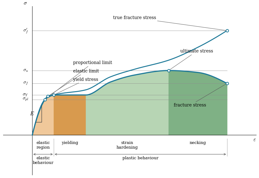
plt.show()8.6.1 holds only in the elastic region, the part of the response in which deformation grows linearly with load and vanishes when the load is removed. Not every material has a well defined elastic region, and some have none worth speaking of, so the law is a model of matter and not a fact about it. Where it applies, the definition of the modulus follows from the definitions of stress and strain,
\[ E := \frac{\Delta\sigma}{\Delta\varepsilon} = \frac{F/A_0}{\Delta L / L_0} = \frac{F L_0}{A_0 \Delta L} \tag{8.6.2}\]
valid as long as \(\Delta L \ll L_0\), which is the same small-deformation assumption that produced 8.5.1. Typical values are \(E \approx 210\,000~\text{MPa}\) for steel, \(68\,000~\text{MPa}\) for aluminium and \(115\,000~\text{MPa}\) for titanium. Printed polymers sit two orders of magnitude lower, around \(2\,000\) to \(3\,500~\text{MPa}\) for PLA and for ABS, the other filament in common use. These figures vary with composition, temperature, strain rate and, for cast or printed material, with position inside the part.
Three ways the model does not fit
Figure 8.6.1 is a ductile metal, and metals are what the machinery of linear elasticity was built around. A printed polymer departs from that picture in three ways, and all of them survive into every number this chapter produces.
It is not linear
A metal has a straight portion. Its slope comes from the stiffness of the atomic bonding, it is very nearly the same on loading and on unloading, and a line fitted anywhere inside that portion gives the same answer. None of it holds for a printed PLA specimen, whose slope falls continuously from the first measurement onwards, as Figure 8.6.5 shows, so no region exists in which a line is uniquely determined, and no slope exists that a second laboratory would recover from a different but equally reasonable choice.
What we report as \(E\) is therefore a secant: the average stiffness between two strains we picked. Quoted without those two strains it means nothing, and this is not a caveat to be tucked into a footnote. It is what the number is.
The stiffness does not come back
Hooke’s law has one parameter and it quietly assumes that parameter stays put. Load a printed specimen well into the curve, then let it go, and it does not retrace the line it came up on. It comes back down a shallower one.
The usual way to carry that is a scalar damage variable \(D\) between zero and one, with the stress written
\[ \sigma = (1 - D)\,E\,\varepsilon \]
so that \(D = 0\) is pristine material at its original stiffness and \(D \to 1\) is material that carries nothing at all. What a test measures while unloading is therefore not \(E\) but the degraded stiffness \((1-D)E\). Writing \(E_1\) for the stiffness the specimen started with and \(E_2\) for the one it comes back on, \(E_2 < E_1\), and the gap between them is the damage the specimen accumulated on the way up.
This has a direct consequence for everything below. A specimen pulled straight to fracture cannot show \(D\) at all. It yields one stiffness, measured near the origin on undamaged material, and by the time the specimen is anywhere near its ultimate stress that number has stopped describing it. Seeing damage requires unloading on purpose, once or several times, and reading the slope on each return.
We have tried and cannot yet resolve it. On a specimen taken up and down seven times, the unloading slopes scatter between roughly 2100 and 2700 MPa and, if anything, rise with the load reached, which is the wrong direction for damage. That is a statement about our measurement rather than about the polymer, and it is the sort of thing a better extensometer would settle.
The point for now is smaller and firm: a single number called the modulus describes the material at one instant of its history, near the beginning. Do not mistake the elastic region for the whole story, and do not mistake \(E\) for a property the specimen carries unchanged to failure.
It is not isotropic
A material that behaves the same in every direction is isotropic, and that is what Hooke’s law with a single \(E\) describes. A rolled steel plate, a drawn aluminium extrusion, a fibre composite and a 3D printed part are all anisotropic to some degree: they have different stiffness and different strength along different axes.
Isotropy is not the same thing as homogeneity. A homogeneous material has the same properties at every point, an isotropic one the same properties in every direction, and a rolled plate is homogeneous but anisotropic. A printed part is neither, since its properties also change from the solid skin to the interior.
For printed parts the anisotropy is severe and it is a design variable rather than a nuisance. Material deposited within a layer is continuous, whereas adjacent layers are joined only where they fused, so a specimen loaded across the layers can fail at a fraction of the strength of one loaded along them. A tensile test therefore characterises a material and a print orientation together, and reporting one without the other says little. This is the reason the specimens in the laboratory are printed to a specified orientation, and the reason that comparing results between groups requires the print parameters to be reported alongside the mechanical data.
A specimen printed standing, with its axis along the build direction, is loaded across every layer at once, and what it measures is layer adhesion, the strength of the bond between layers. Partial infill raises a related problem. A specimen printed with \(20\,\%\) infill is a solid skin around a sparse lattice, and the force divided by its outer area gives an apparent stress: a property of that printed structure and not of the material. The laboratory specimens are printed at \(100\,\%\) infill so that the outer area is the area that carries the load.
A standard written for a different process
ISO 527 is the tensile standard for plastics and it is a good one. ISO 527-2 fixes the test conditions for moulding and extrusion plastics, with specimens moulded to shape or machined from moulded plate [1]. There is the mismatch, and it is worth stating precisely because the imprecise version is easy to refute: the material class is right, the manufacturing route is not ours. A moulded bar is dense, close enough to isotropic, and carries a skin the process gives it. A printed bar is a bonded assembly of extruded roads with a deliberate internal architecture and a skin whose thickness is a slicer setting.
That is a reason to be careful with the result. It is not a reason to abandon the standard, and the argument for keeping it has nothing to do with whether it is physically true.
A testing standard exists so that two laboratories get the same number from the same material. Because ISO 527 is the established way to test plastics, essentially every published modulus you might compare your printed part against was produced with it. Measure some other way and your number may well be closer to the truth, and it will also be incomparable with every datasheet, every supplier figure and every other student group. A value that is right and alone is worth less than a value that is approximate and shared.
The standard is also much more than a strain window. It prescribes how the specimen is gripped and aligned, how much prestress may be present before the measurement starts, what class of extensometer is required, and what speed the test runs at. Those clauses are not decoration: they are what makes the window work. Criticising the window while ignoring the rest is not a criticism of the standard, it is a description of a test that did not follow it, and the end of this chapter applies that test to our own procedure before it applies it to anything else.
A standard does exist for our process. ISO/ASTM 52903-2 covers material extrusion of plastics and includes guidance on building and testing specimens so that direction dependent properties are captured [2]. It prescribes no fit window, so it does not settle the question this chapter is about, but it is where to start on specimen design and on what to report alongside a number.
Why compute a modulus at all
If the material is neither linear nor isotropic, fitting a linear isotropic constant to it invites the objection that the result describes nothing. The objection is sound and the answer is short: no part can be sized without a stiffness. Deflection under load, buckling, natural frequency and every finite element model require one, and a number carrying its conditions is worth more than no number at all.
There is a second answer, and for a student it is the more useful one. Fitting a linear model to a material that does not obey it is not a search for a hidden true value. It is an exercise in taking awkward data, a prescribed procedure and a model known to be wrong, and producing from them a number you are willing to defend. That is most of engineering.
What the objection does rule out is treating the result as a constant of the material in the way \(210\,000~\text{MPa}\) is a constant for steel. For a printed part the stiffness is a property of the material, the print orientation, the print settings and the strain range over which it was measured. All four belong in the report, and a value quoted without them cannot be checked, compared or reused.
The tensile test
A real record looks less tidy than Figure 8.6.1. Figure 8.6.2 is one, a printed polymer specimen taken to failure on our own machine, with the elastic line fitted rather than drawn on by hand.
Code
def read_utm(path):
    """Read a UTM export: header comments into a dict, columns into arrays."""
    meta, rows, names = {}, [], None
    for line in open(path, encoding='utf-8'):
        line = line.rstrip('\n')
        if line.startswith('#'):
            body = line[1:].strip()
            if ':' in body:
                key, value = body.split(':', 1)
                meta[key.strip()] = value.strip()
        elif line.strip():
            if names is None:
                names = line.split(',')
            else:
                rows.append(line.split(','))
    table = np.array(rows, dtype=float)
    return meta, {name: table[:, i] for i, name in enumerate(names)}


meta, col = read_utm('testData/UTM_Test_20260830_122259.csv')

tracked = (col['DIC_Blobs'] == 2) & (col['DIC_Cauchy'] != 0.0)
eps_m, sigma_m = col['DIC_Cauchy'][tracked], col['Stress_MPa'][tracked]

fit = (eps_m >= 0.0005) & (eps_m <= 0.0025)               # the ISO 527 strain window
E_m, b_m = np.polyfit(eps_m[fit], sigma_m[fit], 1)
i_u = np.argmax(sigma_m)

fig, ax = plt.subplots(figsize=(7.4, 5.0))
ax.plot(col['DIC_Cauchy'][~tracked]*100, col['Stress_MPa'][~tracked], 'x', ms=4,
        color='#C25B4E', alpha=.55, label=f'markers lost ({(~tracked).sum()} points)')
ax.plot(eps_m*100, sigma_m, '.', ms=3, color='#236B8E', label='measured')
ax.plot(eps_m[fit]*100, sigma_m[fit], '.', ms=5, color='#C98A2B', label='ISO 527 fit window')
line = np.array([0, 0.0125])
ax.plot(line*100, E_m*line + b_m, '--', lw=1.2, color='k',
        label=f'elastic fit, $E$ = {E_m:.0f} MPa')
ax.plot(eps_m[i_u]*100, sigma_m[i_u], 'o', ms=8, mfc='none', mec='k', mew=1.4)
ax.annotate(f'$R_m$ = {sigma_m[i_u]:.1f} MPa', (eps_m[i_u]*100, sigma_m[i_u]),
            xytext=(8, -4), textcoords='offset points', fontsize=9)
ax.set_xlabel(r'engineering strain $\varepsilon$  (%)')
ax.set_ylabel(r'engineering stress $\sigma$  (MPa)')
ax.set_xlim(-0.15, 3.2); ax.set_ylim(-2, 48)
ax.legend(fontsize=8.5, loc='lower right')
ax.grid(alpha=.25)
plt.tight_layout()
plt.show()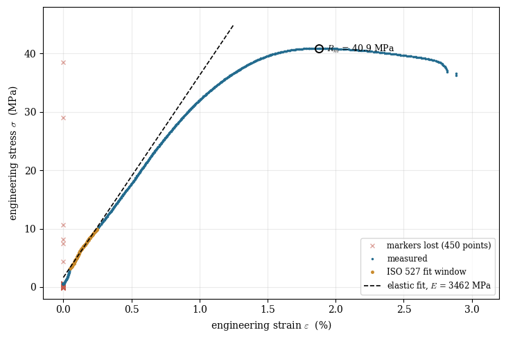
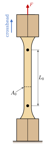
The tensile test is the experiment that produces \(E\) and everything else on Figure 8.6.1. A specimen of known cross section is gripped at both ends and pulled apart at a controlled rate while the machine records the force \(F\) it applies and the extension \(\Delta L\) of a gauge length \(L_0\). The specimen is waisted so that failure occurs in the middle rather than in the grips, which is why tensile specimens have the dogbone shape.
For plastics the shape is fixed by ISO 527-2 [3], and the specimens in our laboratory are its type 1A, the multipurpose specimen, with the dimensions of Table 8.6.1. A parallel portion of width \(b_1\) joins the wider grip ends \(b_2\) through a radius \(r\) on each side. The radius is far larger than the step \((b_2 - b_1)/2 = 5~\text{mm}\), so the arc does not turn a quarter circle into a shoulder face. It leaves the parallel portion tangentially and meets the grip end at an angle, after a horizontal run of \(\sqrt{r^2 - (r - 5)^2} \approx 14.7~\text{mm}\), which with \(l_1 = 80~\text{mm}\) puts the grip ends \(l_2 \approx 109~\text{mm}\) apart.
| Dimension | Symbol | Value [mm] |
|---|---|---|
| Overall length | \(l_3\) | \(\geq 170\) |
| Length of the narrow parallel portion | \(l_1\) | \(80 \pm 2\) |
| Radius | \(r\) | \(24 \pm 1\) |
| Distance between the broad parallel portions | \(l_2\) | \(104\) to \(113\) |
| Width at the ends | \(b_2\) | \(20.0 \pm 0.2\) |
| Width of the narrow portion | \(b_1\) | \(10.0 \pm 0.2\) |
| Thickness | \(h\) | \(4.0 \pm 0.2\) |
| Gauge length | \(L_0\) | \(75.0 \pm 0.5\) |
| Initial distance between the grips | \(L\) | \(115 \pm 1\) |
The large radius keeps the specimen from breaking at the transition. The notebook below computes the stress in the type 1A specimen by the finite element method, with the dimensions of Table 8.6.1 and \(30~\text{MPa}\) in the parallel portion. The peak sits on the arc just before it joins the parallel portion and is \(12\%\) above the nominal stress, and within two millimetres of the join the stress is within one percent of nominal. The gauge length \(L_0 = 75~\text{mm}\) lies inside the \(80~\text{mm}\) parallel portion, where the stress is uniform and one cross section describes the whole of it.
The machine measures force and displacement, but neither is a material property: both depend on how big the specimen happens to be. Dividing by the original cross-sectional area \(A_0\) and the original gauge length \(L_0\) removes the geometry and leaves the engineering stress and engineering strain
\[ \sigma = \frac{F}{A_0}, \qquad \varepsilon = \frac{\Delta L}{L_0} \tag{8.6.3}\]
which are properties of the material alone. Both use the original geometry, which is why they are called engineering rather than true quantities. As the specimen stretches its cross section shrinks, so the true stress on the actual area is higher than the engineering stress, and the difference becomes large once necking begins. For determining the elastic constants the distinction does not matter, because the strains involved are a fraction of a percent.
Reading the curve
Four quantities are normally extracted from a test record. The Young’s modulus is the slope of the initial straight portion. The yield strength marks the end of elastic behaviour. The ultimate tensile strength \(R_m\) is the highest engineering stress the specimen reaches, and the elongation at break is the strain at which it separates, a measure of ductility.
These numbers measure four different properties, and a material can score high on one and low on another. A strong material has a high yield or ultimate strength, a stiff material a high Young’s modulus, and a ductile material reaches a large plastic strain before fracture. Toughness is the energy per unit volume absorbed up to fracture, the area under the stress-strain curve, so it needs strength and ductility together. Glass is stiff but not ductile, and therefore not tough, while annealed copper is ductile without being strong. The straight portion of Figure 8.6.1 ends at the proportional limit, the stress at which the curve stops being linear. It is a stress, not a stiffness, and it lies at or below the yield strength.
The yield strength needs care because most materials do not yield abruptly. Mild steel is the exception, showing a distinct upper and lower yield point that can simply be read off. Aluminium, titanium and most polymers curve over gradually, with no point that is obviously the end of the elastic region. The convention adopted by the testing standards is the offset yield strength \(R_{p0.2}\): draw a line parallel to the elastic slope but shifted to the right by a plastic strain of \(0.2\%\), and take the stress where that line crosses the measured curve. The definition is arbitrary, which is exactly why it is standardised: everyone who follows it gets the same number from the same data. The construction and the \(0.2\%\) value are prescribed for metals by ISO 6892-1 [4] and ASTM E8 [5], and for plastics by ISO 527-1 [1], which also fixes the strain window used to fit the modulus.
⚠ Note
The offset construction depends on the fitted modulus. An error in \(E\) shifts the offset line and moves \(R_{p0.2}\) with it, so the modulus must be fitted before the yield strength is read, not the other way around.
Example 1: Processing a test record
The evaluation is four steps. First read the file and throw away the samples the instrument could not measure. Second fit a straight line to the elastic part and read its slope as \(E\). Third shift the strain axis so that the fitted line passes through the origin. Fourth construct the offset line and find where it crosses the measurement.
We work through them on one specimen of printed PLA, nominal section \(80~\text{mm}^2\), pulled to fracture on the laboratory machine, Figure 8.6.3.
Step 1: The data
The machine writes a block of # comment lines carrying the specimen area, the gauge length and the load at which the strain measurement was zeroed, then one header row, then the data. Because it has already divided force by the original area and marker separation by its original value, the two columns we need are 8.6.3 ready made.
The area in that header is the one typed into the machine before the test. It should be the measured area, width times thickness of the gauge section taken with a caliper, and not the nominal area of the CAD model. Printed specimens do not hold their drawn dimensions, and a section a few percent off moves every stress, and \(E\) with it, by the same few percent. This record was run on the nominal \(80~\text{mm}^2\), so for a measured area \(A\) its stresses scale by \(80~\text{mm}^2/A\).
Two columns carry strain and only one of them belongs to the material. DIC_Cauchy is the separation of two markers on the specimen, tracked by a camera, relative to their separation at zero load. Motor_Strain is crosshead travel divided by gauge length, and the crosshead also moves the frame, the fixture, the grips and the shoulders of the specimen, so it overstates the strain of the gauge section by a factor of three or more. Use DIC_Cauchy.
The camera also drops frames. When the tracker cannot see exactly two markers it writes a blob count other than two, and when a frame is lost it writes a strain of exactly zero. Both appear in a raw plot as a stripe of points stacked on the \(\varepsilon = 0\) axis, and both have to go before anything is fitted.
path = 'testData/UTM_Test_20260830_122259.csv'

n_header = sum(1 for line in open(path) if line.startswith('#'))
data = np.genfromtxt(path, delimiter=',', skip_header=n_header, names=True)

tracked = (data['DIC_Blobs'] == 2) & (data['DIC_Cauchy'] != 0.0)
sigma = data['Stress_MPa'][tracked]        # engineering stress [MPa]
eps = data['DIC_Cauchy'][tracked]          # engineering strain [-]

ltx(r"\text{rows in the file} &=", len(tracked),
    r"\\ \text{rows with both markers tracked} &=", int(tracked.sum()), aligned=True)
\[ \begin{aligned}\text{rows in the file} &=1229\\ \text{rows with both markers tracked} &=779\end{aligned} \]
Step 2: Fit the modulus
The modulus is the slope of the elastic part, and the only real decision in the whole evaluation is which points belong to it. Too few and the slope is noise. Too many and the line is dragged down as the curve bends over.
A printed polymer makes this harder than the idealised picture suggests, because it has no straight portion worth the name: the slope falls continuously from the first measurement onwards. There is no window that is right in the sense of capturing a genuinely linear region, only windows that are defensible and reproducible.
We use the one the standard prescribes. ISO 527-1 fits between \(0.05\%\) and \(0.25\%\) strain [1], and we follow it for the reason given above: it is what everyone else uses, so the number can be compared with somebody else’s. How well that window survives a printed specimen, and an alternative we have been testing, are taken up at the end of the chapter.
Within the window we fit the line
\[ \sigma = E\varepsilon + b, \qquad \min_{E,\,b}\sum_{0.0005\,\le\,\varepsilon_i\,\le\,0.0025}\left(\sigma_i - E\varepsilon_i - b\right)^2 \]
window = (eps >= 0.0005) & (eps <= 0.0025)     # the ISO 527-1 strain window
E_fit, intercept = np.polyfit(eps[window], sigma[window], 1)

i_u = np.argmax(sigma)                          # the ultimate point, needed further down
R_m, eps_u = sigma[i_u], eps[i_u]

ltx(r"E &=", E_fit, r"~\text{MPa}",
    r"\\ \text{points used} &=", int(window.sum()),
    r"\\ R_m &=", R_m, r"~\text{MPa}",
    r"\\ \varepsilon_u &=", 100*eps_u, r"~\%", aligned=True)
\[ \begin{aligned}E &=3462.27~\text{MPa}\\ \text{points used} &=83\\ R_m &=40.93~\text{MPa}\\ \varepsilon_u &=1.88~\%\end{aligned} \]
Step 3: Remove the toe
The fitted line does not pass through the origin. Its intercept is the signature of the toe region, the initial slack while the grips settle and the specimen straightens, which adds extension without adding load. Anything that happened before the strain measurement was zeroed ends up there too: this file records that the camera was zeroed after a preload of \(49~\text{N}\), which on \(80~\text{mm}^2\) is \(0.61~\text{MPa}\) the specimen already carried at the moment it was told its strain was zero. That is about a third of the \(1.64~\text{MPa}\) intercept, and comfortably inside the prestress the standard allows, which is \(E_t/2000\) or \(1.7~\text{MPa}\) here.
The toe belongs to the fixture and to the procedure, not to the material, so we slide the strain axis until the fitted line does pass through the origin. Since \(E\varepsilon + b = E(\varepsilon + b/E)\), the corrected strain is
\[ \varepsilon_c = \varepsilon + \frac{b}{E} \]
eps_corrected = eps + intercept/E_fitStep 4: The offset construction
The offset line is the elastic line moved to the right by a plastic strain of \(0.002\),
\[ \sigma_\text{off} = E(\varepsilon_c - 0.002) \]
and \(R_{p0.2}\) is the measured stress where the difference \(d_i = \sigma_i - \sigma_{\text{off},i}\) changes sign. Between the two points \(i\) and \(i+1\) that bracket the sign change we interpolate linearly,
\[ t = \frac{-d_i}{d_{i+1} - d_i}, \qquad R_{p0.2} = \sigma_i + t(\sigma_{i+1} - \sigma_i) \]
A record that rises to a peak and then softens crosses the offset line more than once, so we take the first crossing beyond the fit window and not the last.
offset_line = E_fit * (eps_corrected - 0.002)
difference = sigma - offset_line

crossings = np.where(np.diff(np.sign(difference)))[0]            # every sign change
crossing = crossings[eps_corrected[crossings] > 0.0025][0]        # first beyond the window
t = -difference[crossing] / (difference[crossing+1] - difference[crossing])

R_p02 = sigma[crossing] + t*(sigma[crossing+1] - sigma[crossing])
eps_last = eps_corrected[-1]              # last strain read before the markers were lost

ltx(r"E &=", E_fit, r"~\text{MPa}",
    r"\\ R_{p0.2} &=", R_p02, r"~\text{MPa}",
    r"\\ R_m &=", R_m, r"~\text{MPa}",
    r"\\ \varepsilon_{\text{last}} &=", 100*eps_last, r"~\%", aligned=True)
\[ \begin{aligned}E &=3462.27~\text{MPa}\\ R_{p0.2} &=35.41~\text{MPa}\\ R_m &=40.93~\text{MPa}\\ \varepsilon_{\text{last}} &=2.93~\%\end{aligned} \]
Reading the result
The evaluation gives a modulus of \(3462~\text{MPa}\), an offset yield strength of \(35.4~\text{MPa}\) and an ultimate strength of \(40.9~\text{MPa}\).
Two of those deserve comment. The yield strength sits at \(87\%\) of the ultimate, which looks wrong and is not: a curve that bends over this gradually is not met by a line offset by \(0.2\%\) of plastic strain until the material is close to its peak. And the last strain we can report is \(2.9\%\), which is not the elongation at break. The markers separate beyond what the tracker will follow at the moment the specimen fails, so an optical extensometer measures everything except the quantity that needs the specimen to be in one piece.
Figure 8.6.4 shows the record with both constructions drawn on it.
Code
fig, (ax, axz) = plt.subplots(1, 2, figsize=(11, 4.5))

# Left: the whole record with both results marked
ax.plot(100*eps_corrected, sigma, 'k', lw=1.2, label='measurement')
ax.plot(100*eps_corrected, offset_line, 'b--', lw=1, label=r'$0.2\%$ offset line')
ax.plot(100*eps_corrected, E_fit*eps_corrected, 'g:', lw=1.4, label='fitted elastic slope')
ax.plot(100*eps_corrected[i_u], R_m, 'ro')
ax.annotate(rf'$R_m$ = {R_m:.1f} MPa', (100*eps_corrected[i_u], R_m),
            xytext=(6, -12), textcoords='offset points', fontsize=9)
ax.plot(100*(eps_corrected[crossing] + t*np.diff(eps_corrected)[crossing]), R_p02, 'bo')
ax.annotate(rf'$R_{{p0.2}}$ = {R_p02:.1f} MPa',
            (100*eps_corrected[crossing], R_p02),
            xytext=(-8, 12), textcoords='offset points', fontsize=9, ha='right', color='b')
ax.set_xlim(0, 100*eps_corrected.max()*1.05)
ax.set_ylim(0, 1.18*R_m)
ax.set_title('Full record', fontsize=11)
ax.legend(loc='lower right', fontsize=9)

# Right: the elastic region, showing which points were actually fitted
axz.plot(100*eps_corrected, sigma, 'k', lw=1.2, label='measurement')
axz.plot(100*eps_corrected[window], sigma[window], 'o', ms=3, color='#C98A2B',
         label=r'fitted points, ISO 527 window')
axz.plot(100*eps_corrected, E_fit*eps_corrected, 'g:', lw=1.4, label='fitted elastic slope')
axz.set_xlim(0, 0.45)
axz.set_ylim(0, 16)
axz.set_title('The elastic region and the fit window', fontsize=11)
axz.legend(loc='lower right', fontsize=9)

for a in (ax, axz):
    a.grid(True)
    a.set_xlabel(r'$\varepsilon$ [%]')
    a.set_ylabel(r'$\sigma$ [MPa]')

plt.tight_layout()
plt.show()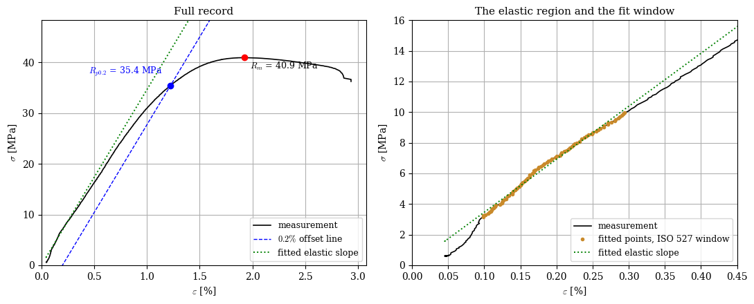
The zoomed view on the right is where the judgment lies. The offset line runs parallel to the fitted slope, so any error in the fit tilts it, and the crossing then slides along a shallow part of the curve where a small vertical error means a large horizontal one. Two students who fit different windows will report different moduli and, through them, different yield strengths. Reporting the window, the strain source and the specimen geometry alongside the numbers is what makes two sets of results comparable at all.
Choosing the fit window
Everything above rests on the decision made in step 2, and a material with no straight portion offers nothing to make that decision for us. Any window is a convention. The questions are which convention, whether the person quoting a number says which one they used, and whether the rest of the test was run well enough for the question to matter.
Before criticising the standard: what we did not do
ISO 527-1 prescribes much more than the strain window, and our own records do not satisfy all of it. Two clauses matter here and both are measurable from the files.
Prestress. Clause 9.4 requires the specimen to carry a small positive stress before the measurement starts, enough to pull out slack and seat the grips, and caps it at \(\sigma_0 \le E_t/2000\), a prestrain of \(0.05\%\) in the standard’s own words. For the record evaluated above that cap is \(1.7~\text{MPa}\) and the file records \(0.61~\text{MPa}\), so this one complies. Other records in the same folder do not, and the student sets we have seen run up to twice the limit. Too little prestress leaves a toe; too much starts the measurement inside the curve. Both move the modulus.
Test speed. Clause 9.6 requires a strain rate as close as possible to \(1\%\) of the gauge length per minute for modulus measurement. The record above was pulled at \(6~\text{mm/min}\) on an \(80~\text{mm}\) gauge, which is \(7.5\%\) per minute, seven times too fast. Polymers are strain rate sensitive, so this inflates both the modulus and the strength relative to any catalogue value. The standard anticipates the tedium and allows a two speed test: run at \(1\%\) per minute to \(\varepsilon = 0.25\%\), change speed before \(\varepsilon = 0.3\%\), and continue to fracture at whatever rate you like.
None of this excuses the standard’s window on a printed specimen. It does mean that what follows is evidence about our test, and that the first thing to fix is our procedure rather than the standard.
Where the straight part actually is
Figure 8.6.5 takes the record evaluated above and fits a short line at every point along it, so that the local slope can be read directly.
Code
half = 0.0004                                   # half width of the sliding fit, in strain
centres = np.arange(0.0006, 0.0100, 0.0002)
slopes = []
for c in centres:
    near = (eps >= c - half) & (eps <= c + half)
    slopes.append(np.polyfit(eps[near], sigma[near], 1)[0] if near.sum() >= 8 else np.nan)

fig, ax = plt.subplots(figsize=(7, 4.2))
ax.plot(100*centres, slopes, 'o-', ms=3, lw=1.2, color='#236B8E')
ax.axvspan(0.05, 0.25, color='#C25B4E', alpha=.14, label='ISO 527 window')
ax.axvspan(100*0.10*eps_u, 100*0.50*eps_u, color='#7A9E3F', alpha=.18,
           label=r'$0.10\,\varepsilon_u$ to $0.50\,\varepsilon_u$')
ax.axhline(E_fit, color='k', ls='--', lw=0.9, label=f'fitted $E$ = {E_fit:.0f} MPa')
ax.set_xlabel(r'strain $\varepsilon$ (%)')
ax.set_ylabel(r'local slope $\mathrm{d}\sigma/\mathrm{d}\varepsilon$ (MPa)')
ax.set_xlim(0, 1.0)
ax.legend(fontsize=9)
ax.grid(alpha=.25)
plt.tight_layout()
plt.show()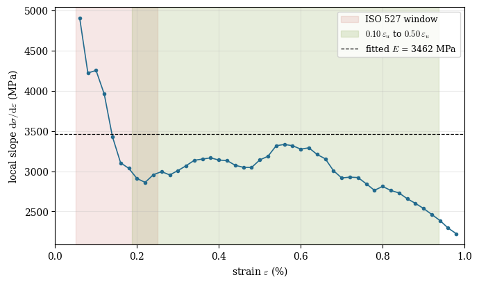
A material does not become \(40\%\) more compliant and then stop. The steep part at the left is the instrument: the optical extensometer resolves strain in steps of about \(0.006\%\), and the ISO window spans only three pixels of marker separation, so the line is being fitted through a staircase. On this record the standard’s window sits inside that artefact, and the plateau between roughly \(0.25\%\) and \(0.65\%\) sits outside it.
That is the honest statement of the problem, and the honest response is not to discard the window. It is to fix the measurement, which means more pixels across the gauge, prestress inside the clause 9.4 limit and the speed clause 9.6 asks for. Until that is done we cannot tell how much of this is the standard and how much is us.
An experiment: a window that scales with the material
In the meantime we have been testing an alternative, and it is reported here as an experiment, not as a recommendation. Instead of fixed strain limits, take the window as a fraction of the strain at which the specimen reaches its ultimate stress,
\[ 0.10\,\varepsilon_u \le \varepsilon \le 0.50\,\varepsilon_u \]
which lands on the same part of the curve whatever the material, and scales itself to something brittle as readily as to something ductile. On the record above it selects \(0.19\%\) to \(0.94\%\), which is the plateau in Figure 8.6.5.
The test of any window is not whether it looks right on one record but whether it gives the same answer on specimens that should be the same. Four were printed and pulled together.
Code
records = ['122259', '123728', '124746', '125231']

def evaluate(rec, lo, hi, by='strain'):
    p = f'testData/UTM_Test_20260830_{rec}.csv'
    n = sum(1 for line in open(p) if line.startswith('#'))
    d = np.genfromtxt(p, delimiter=',', skip_header=n, names=True)
    keep = (d['DIC_Blobs'] == 2) & (d['DIC_Cauchy'] != 0.0)
    e, s = d['DIC_Cauchy'][keep], d['Stress_MPa'][keep]
    peak = np.argmax(s)
    if by == 'strain':      m = (e >= lo) & (e <= hi)
    elif by == 'eps_u':     m = (e >= lo*e[peak]) & (e <= hi*e[peak])
    else:                                              # fraction of the ultimate stress
        m = (s >= lo*s[peak]) & (s <= hi*s[peak]); m[peak+1:] = False
    return np.polyfit(e[m], s[m], 1)[0], s[peak]

methods = [(r"\text{ISO 527, } 0.05\text{ to }0.25\,\%", 0.0005, 0.0025, 'strain'),
           (r"\text{fixed, } 0.25\text{ to }1.00\,\%",   0.0025, 0.0100, 'strain'),
           (r"0.30\,R_m \text{ to } 0.70\,R_m",          0.30,   0.70,   'stress'),
           (r"0.10\,\varepsilon_u \text{ to } 0.50\,\varepsilon_u", 0.10, 0.50, 'eps_u')]

rows = []
for label, lo, hi, by in methods:
    v = np.array([evaluate(r, lo, hi, by)[0] for r in records])
    rows.append(r"%s & %s & %.0f & %.1f\,\%% \\" % (label, ' & '.join(f'{x:.0f}' for x in v),
                                               v.mean(), 100*v.std(ddof=1)/v.mean()))
Rm = np.array([evaluate(r, 0.10, 0.50, 'eps_u')[1] for r in records])
rows.append(r"\hline \text{ultimate strength } R_m & %s & %.1f & %.1f\,\%% \\"
            % (' & '.join(f'{x:.1f}' for x in Rm), Rm.mean(), 100*Rm.std(ddof=1)/Rm.mean()))

ltx(r"\begin{array}{l r r r r r r} \text{fit window} & " +
    ' & '.join(records) + r" & \text{mean} & \text{CV} \\ \hline " +
    ' '.join(rows) + r"\end{array}")
\[ \begin{array}{l r r r r r r} \text{fit window} & 122259 & 123728 & 124746 & 125231 & \text{mean} & \text{CV} \\ \hline \text{ISO 527, } 0.05\text{ to }0.25\,\% & 3462 & 4098 & 4604 & 3772 & 3984 & 12.3\,\% \\ \text{fixed, } 0.25\text{ to }1.00\,\% & 3024 & 2572 & 2457 & 2510 & 2641 & 9.8\,\% \\ 0.30\,R_m \text{ to } 0.70\,R_m & 3112 & 3010 & 3721 & 2868 & 3177 & 11.8\,\% \\ 0.10\,\varepsilon_u \text{ to } 0.50\,\varepsilon_u & 3068 & 2755 & 3034 & 2701 & 2889 & 6.5\,\% \\ \hline \text{ultimate strength } R_m & 40.9 & 40.2 & 40.8 & 39.0 & 40.2 & 2.2\,\% \\\end{array} \]
The four specimens agree on ultimate strength to about two percent. They agree on the modulus to between six and twelve percent depending only on how it was evaluated, and the standard’s window is the worst of the four on this data.
The last column is the coefficient of variation, the standard deviation divided by the mean. It is the natural measure here because the question is not how large the modulus is but how repeatable the procedure that produced it.
What to take from this
Strength is easy to measure and stiffness is hard, and a large part of the difficulty sits in the evaluation and not in the specimen. That is worth carrying into any test you run.
For the laboratory, use the ISO 527 window, and report it alongside the number together with the strain source, the test speed, the prestress and how many specimens were behind it. A modulus without those cannot be checked by anyone, and one measured a different way cannot be compared with anything.
The experiment above is not yet a method. It rests on four specimens of one material on one machine, it has not been tried on a material with a very different \(\varepsilon_u\), and a brittle specimen that fractures at its maximum stress makes \(\varepsilon_u\) mean something different from what it means for a specimen that yields first. It also, being wider, is more exposed to gaps in the strain record than the narrow window it replaces. Treat it as an open question this department is working on, not as an answer.
What is settled is smaller and more useful. There is no true modulus here waiting to be recovered by a sufficiently careful experiment. There is a curve, and there are conventions for reducing it to a number, and on a printed specimen the conventions disagree with one another by more than the specimens disagree among themselves. Following a standard does not make that go away. It does mean that everyone disagrees in the same direction, which is what makes comparison possible at all, and it is why we follow it.
Publish the curve, not the four numbers
This chapter has spent its length turning one curve into four numbers, and every step of that reduction needed a convention: which points are elastic, where the toe ends, what offset defines yield, which strain signal to believe. The numbers are useful. They are also a lossy compression of the measurement, and the losses are not small.
Consider two materials we have tested side by side. Printed PLA reaches an ultimate strength of \(44.1~\text{MPa}\); cast acrylic reaches \(46.0~\text{MPa}\), within four percent of it. Their moduli sit within about a quarter of each other. In a table of scalars they are near neighbours. In fact the acrylic runs almost straight from the origin to a brittle fracture at \(1.5\%\) strain, while the PLA bends through a knee and rolls over to a rounded maximum near \(2\%\) before it softens. One of them warns you before it fails and one does not. A designer choosing between them on \(E\) and \(R_m\) alone would have no way to know which.
The damage variable of the previous section is invisible in the same way. So is the shape of the yield transition, the presence or absence of a knee, the strain rate the test was run at, and every disagreement between specimens that the mean quietly absorbs.
There is a second loss, and it is the one this chapter has been living with. A published modulus cannot be re-evaluated. If a colleague reports \(3462~\text{MPa}\) for a printed PLA, we cannot ask what it would have been over a different strain window, or what the curve looked like where the window sat, or whether the low strain region was instrument or material. The entire argument of this chapter would be settled in an afternoon if the curves behind a few hundred published moduli were available. They are not, and so everyone re-derives the same uncertainty privately.
The remedy is cheap to the point of being embarrassing. A complete tensile record is a few tens of kilobytes of text, smaller than the PDF datasheet that summarises it. Publishing it asks almost nothing and returns a great deal:
anyone can re-evaluate under their own convention, or under a standard that did not exist when the test was run; anyone can fit a model the original authors were not using, whether that is damage, viscoelasticity or something with more parameters than Hooke’s law has; and anyone can pool records across laboratories and find out how much of the published scatter is the material and how much is the method. None of that is possible from a scalar.
So alongside the number, publish the record that produced it: force and extension as measured, the specimen geometry, the gauge length, the strain source, the test speed, the prestress, and for a printed specimen the print parameters and orientation. State which convention produced the scalar so that it can be reproduced, and give the data so that it need not be.
We ask students to do this in the laboratory, and the reason is not pedagogical tidiness. It is that a number without its curve cannot be checked, and a discipline that publishes only numbers has agreed in advance not to check itself.
References
[1]
ISO 527-1:2019 Plastics – Determination of tensile properties – Part 1: General principles. Geneva, Switzerland: International Organization for Standardization; 2019.
[2]
ISO/ASTM 52903-2:2020 Additive manufacturing – Material extrusion-based additive manufacturing of plastic materials – Part 2: Process equipment. Geneva, Switzerland: International Organization for Standardization; ASTM International; 2020.
[3]
ISO 527-2:2012 Plastics – Determination of tensile properties – Part 2: Test conditions for moulding and extrusion plastics. Geneva, Switzerland: International Organization for Standardization; 2012.
[4]
ISO 6892-1:2019 Metallic materials – Tensile testing – Part 1: Method of test at room temperature. Geneva, Switzerland: International Organization for Standardization; 2019.
[5]
ASTM E8/E8M-22 Standard Test Methods for Tension Testing of Metallic Materials. West Conshohocken, PA, USA: ASTM International; 2022.