“Die Reißwerkzeuge hat er immer bei der Hand, das Zeichnen ist seine Sprache.”
“He always has his drawing instruments to hand; drawing is his language.”
— Karl Culmann, Die graphische Statik, 1866, our translation
The rod equation of Chapter 8.12 governs a single member lying along a line. A truss is many such members pointing in many directions, pinned together at their ends. Nothing new is needed physically, since each rod still obeys \(\delta = NL/EA\), but the bookkeeping changes: each rod has its own axis, while the joints they share move in a common frame. This chapter builds the machinery that translates between the two, by hand and on a structure small enough to check every entry.
What a truss is
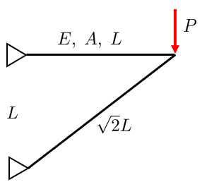
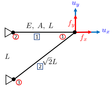
Figure 8.14.1 shows the simplest case. Two rods meet at a pinned joint, the other two ends are fixed, and a force \(P\) acts at the joint. The pins are assumed frictionless and moment free, so each rod can carry only axial force, which is why loads may be applied at joints and nowhere else. In two dimensions each joint can translate in \(x\) and \(y\), so it has two degrees of freedom.
A cable or rope also carries only axial force, but only in tension: under compression it slackens and carries nothing, so it cannot stand in for a rod whose force may change sign. The rods must also be arranged so that no joint can move without some rod changing length. A rectangle of four rods without a diagonal fails this, and a truss that can move that way is a mechanism, neither statically determinate nor statically indeterminate but unstable.
Figure 8.14.1: A simple truss: two rods, one loaded joint and two supports.
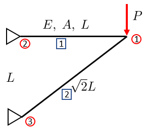
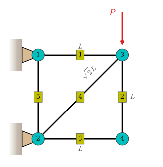
The analysis begins by numbering every rod and every joint, since every quantity below is indexed by one or the other. Figure 8.14.2 fixes rods in squares and nodes in circles, a convention worth keeping because the two sets of numbers are used in different equations and confusing them is the commonest source of error.
Figure 8.14.2: Rods numbered in squares, nodes in circles.
Each rod carries four quantities of interest: the normal force \(N_i\), the normal stress \(\sigma_i\), the strain \(\varepsilon_i\) and the deformation \(\delta_i\). Each node carries two: the nodal force \(f_j\) and the nodal displacement \(u_j\). The question a designer asks is whether the structure can carry the load, which turns into requirements on the maximum stress, the maximum displacement and the reaction forces at the supports.
Counting rods and equations
Whether equilibrium alone fixes the rod forces can be decided by counting, before any joint is cut free. Each pinned joint gives two equilibrium equations, one in \(x\) and one in \(y\), so a plane truss with \(j\) joints has \(2j\) equations. The unknowns are the \(m\) rod forces and the \(r\) support reactions, two at a pin support and one at a roller. Comparing the two counts gives three cases,
and in the last case the surplus \(m + r - 2j\) is the degree of static indeterminacy, the number of compatibility conditions that must be added to equilibrium before the rod forces can be found.
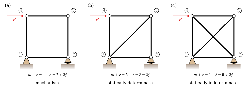
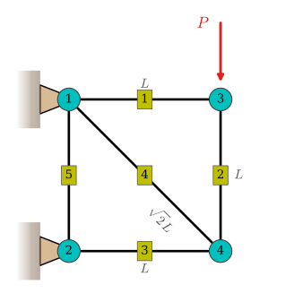
Figure 8.14.3 applies the count to a square on a pin and a roller, with \(j = 4\) joints, \(r = 3\) reactions and therefore \(2j = 8\) equations. Without a diagonal, (a) has seven unknowns for eight equations. One equation cannot be met for a general load, and the square folds into a parallelogram. One diagonal, (b), splits the square into two triangles, the smallest arrangement that keeps it rigid, and the eight unknowns follow from the eight equations. A second diagonal, (c), adds a ninth unknown. The load now has two paths across the square, and how it divides between the two diagonals depends on their stiffnesses \(EA/L\), which equilibrium does not contain. The three-rod truss of Example 1 below counts the same way: \(j = 4\), \(m = 3\) and \(r = 6\), since nodes 2, 3 and 4 are pinned, so \(m + r = 9 > 8\) and it is once statically indeterminate.
Figure 8.14.3: Counting unknowns against equations for a square on a pin and a roller, \(j = 4\) and \(r = 3\). (a) Without a diagonal the square is a mechanism. (b) One diagonal makes it statically determinate. (c) Two diagonals make it statically indeterminate to the first degree.
The count is necessary but not sufficient. It says whether there are enough rods and reactions, not whether they sit in the right places. Turn the roller of (b) so that it pushes horizontally: the count is still eight, but all three reactions now pass through the pin at node 1, nothing resists a rotation about it, and the truss is a mechanism. The geometric check is to build the truss from triangles. Start from one triangle and attach each new joint with two rods that are not in line, and support the whole on reactions that neither meet in one point nor are all parallel. A truss built that way and passing 8.14.1 is statically determinate.
The Golden Quad for a truss
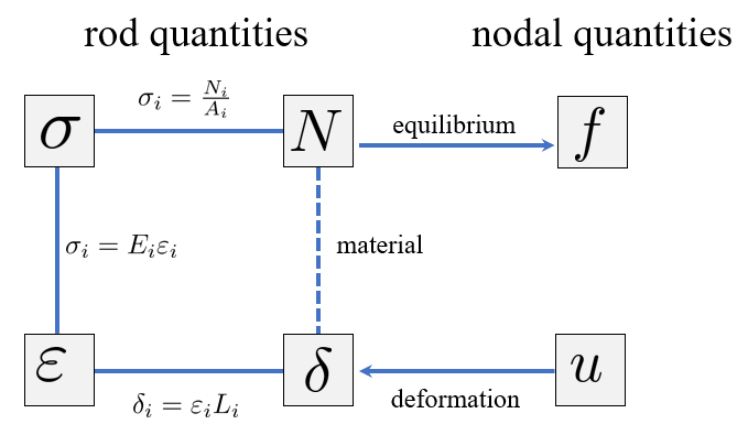
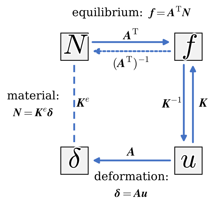
Figure 8.14.4 is Figure 8.11.1 redrawn with the truss quantities in place. The internal, rod-level quantities are on the left, the external, node-level quantities on the right, and the same three relations join them.
Figure 8.14.4: The three relations of Chapter 8.11, written for a truss.
Reading the arrows, equilibrium connects the rod forces to the nodal forces, the material relation connects the strains to the stresses through \(\sigma_i = E_i\varepsilon_i\), and the deformation relation connects the nodal displacements to the rod deformations through \(\delta_i = \varepsilon_i L_i\). Combining the last two gives what each rod contributes,
which is 8.11.5, itself the simplest solution of the boundary value problem 8.12.5 with no body load. Because we are solving that problem member by member rather than as a field over the structure, this approach is called the direct method: it attacks the differential equation directly, at the cost of only working for members whose solution we already know.
Figure 8.14.5: Boundary conditions and the degrees of freedom of the loaded node.
For the structure in Figure 8.14.5 the supports impose \(u_2^x = u_2^y = u_3^x = u_3^y = 0\), and node 1 is free with two degrees of freedom. We collect them, and the nodal loads, into vectors
\[
\bm u = \begin{bmatrix} u_1^x \\ u_1^y \end{bmatrix},
\qquad
\bm f = \begin{bmatrix} f_1^x \\ f_1^y \end{bmatrix}
\]
leaving the known value \(f_1^y = -P\) to be substituted at the very end. Working symbolically for as long as possible is deliberate: the structure of the answer is visible in the symbols and invisible in the numbers.
Three matrices
The goal is a relation between the loads and the displacements of the form \(\bm K \bm u = \bm f\), from which \(\bm u = \bm K^{-1}\bm f\). Figure 8.14.6 shows how the three relations produce it.
Figure 8.14.6: The three matrices and the two routes between loads and displacements.
The deformation relation is a matrix \(\bm A\) that turns nodal displacements into rod deformations,
\[
\bm\delta = \bm A\,\bm u
\tag{8.14.3}\]
The material relation is a diagonal matrix \(\bm K^e\) holding each rod’s stiffness from 8.14.2,
\[
\bm N = \bm K^e\,\bm\delta
\tag{8.14.4}\]
and equilibrium of each joint turns rod forces into nodal forces,
\[
\bm f = \bm A^\mathsf{T}\,\bm N
\tag{8.14.5}\]
The transpose in 8.14.5 is a consequence of energy conservation: the work done by the nodal forces on the nodal displacements must equal the work done by the rod forces on the rod deformations, \(\bm f^\mathsf{T}\bm u = \bm N^\mathsf{T}\bm\delta = \bm N^\mathsf{T}\bm A\bm u\), for every \(\bm u\). The practical consequence is that we may derive whichever of \(\bm A\) and \(\bm A^\mathsf{T}\) is easier and simply transpose it.
Chaining the three gives the structural stiffness matrix
\[
\boxed{\bm f = \bm A^\mathsf{T}\bm N = \bm A^\mathsf{T}\bm K^e\bm\delta = \underbrace{\bm A^\mathsf{T}\bm K^e\bm A}_{\bm K}\,\bm u}
\tag{8.14.6}\]
which is symmetric, because \(\bm K^e\) is diagonal and \((\bm A^\mathsf{T}\bm K^e\bm A)^\mathsf{T} = \bm A^\mathsf{T}\bm K^e\bm A\). Once \(\bm u\) is known, the rod quantities follow by walking the arrows backwards: \(\bm\delta = \bm A\bm u\), then \(\bm N = \bm K^e\bm\delta\), then \(\sigma_i = N_i/A_i\).
Example 1: A three-rod truss
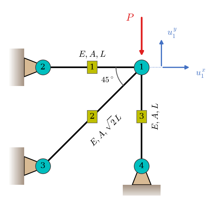
Figure 8.14.7 shows the structure. Rod 1 is horizontal with length \(L\), rod 2 runs diagonally at \(45^\circ\) with length \(\sqrt2 L\), and rod 3 is vertical with length \(L\). All three have the same \(E\) and \(A\). Node 1 is free and carries the load; nodes 2, 3 and 4 are fixed.
Figure 8.14.7: The three-rod truss. Node 1 is free with displacements \(u_1^x\) and \(u_1^y\).
We follow a fixed sequence: number the rods and nodes, choose a coordinate system, here the usual one with \(x\) to the right and \(y\) upwards, introduce the displacement and load vectors, introduce the rod vectors, build \(\bm A\) or \(\bm A^\mathsf{T}\), build \(\bm K^e\), assemble, and solve. The vectors are
\[
\bm u = \begin{bmatrix} u_1^x \\ u_1^y \end{bmatrix},
\qquad
\bm f = \begin{bmatrix} f_1^x \\ f_1^y \end{bmatrix},
\qquad
\bm\delta = \begin{bmatrix}\delta_1\\\delta_2\\\delta_3\end{bmatrix},
\qquad
\bm N = \begin{bmatrix}N_1\\N_2\\N_3\end{bmatrix}
\]
Building A by unit displacements
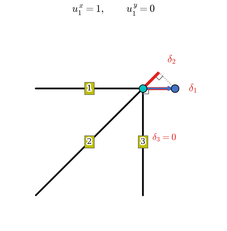
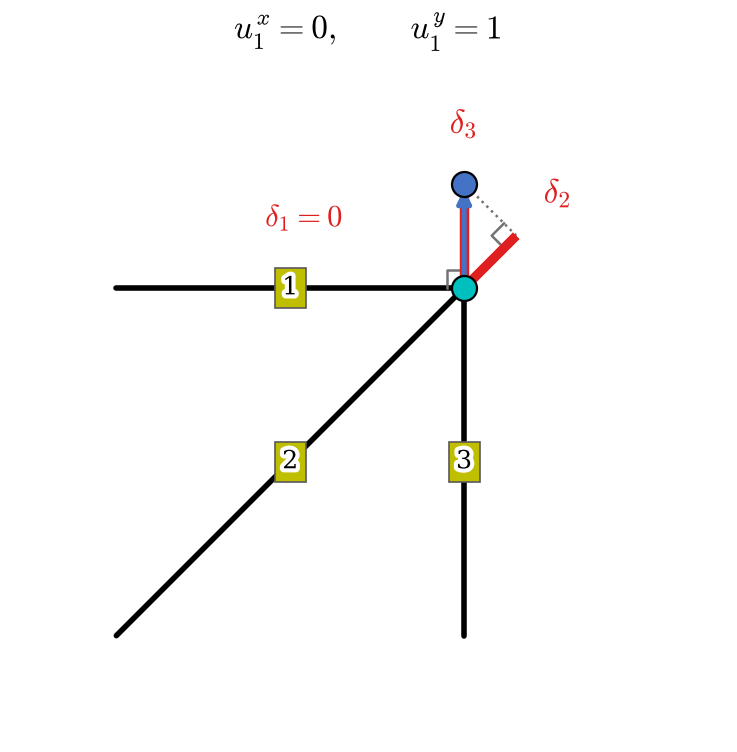
Read 8.14.3 column by column. Setting \(\bm u = [1, 0]^\mathsf{T}\) gives \(\bm\delta\) equal to the first column of \(\bm A\), and \(\bm u = [0, 1]^\mathsf{T}\) gives the second. Each column is therefore the set of rod deformations produced by moving the free node one unit in one coordinate direction, which is something we can read straight off a deformation figure.
The small-deformation assumption is what makes this legitimate. Because the displacements are infinitesimal compared with the rod lengths, each rod may be treated as merely translated, staying parallel to its original direction, and its deformation is the projection of the nodal displacement onto its own axis.
Figure 8.14.8: Unit displacement in \(x\)
Figure 8.14.9: Unit displacement in \(y\)
Moving node 1 one unit in \(x\), as in Figure 8.14.8, stretches rod 1 by its full length, stretches rod 2 by the projection \(\cos 45^\circ = 1/\sqrt2\), and does nothing to the vertical rod 3,
Moving it one unit in \(y\), as in Figure 8.14.9, leaves the horizontal rod 1 unchanged, stretches rod 2 by \(\sin 45^\circ\) and stretches rod 3 by its full length,
Every entry here is positive because moving the joint upwards pulls on both of the rods that hang below it. Signs do matter, and they will appear as soon as the load is applied downwards. Assembling the two columns,
and note that not one material property or cross-sectional area appears in it. The matrix \(\bm A\) is purely geometric.
Building the same matrix by joint equilibrium
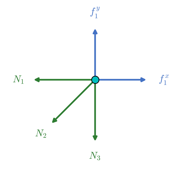
The alternative route reads 8.14.5 instead, and it is the classical method of joints. Isolate node 1 and write force equilibrium in the two coordinate directions, with the rod forces drawn positive in tension so that each pulls the joint towards the far end of its rod.
E, A, L, P = sp.symbols('E A L P', positive=True)r2 = sp.sqrt(2)A_mat = sp.Matrix([[1, 0], [1/r2, 1/r2], [0, 1]])K_e = (E*A/L) * sp.diag(1, 1/r2, 1)K = sp.simplify(A_mat.T * K_e * A_mat)ltx(r"\bm A &=", A_mat, r",\quad \bm K^e =", K_e,r"\\\bm K &= \bm A^\mathsf{T} \bm K^e \bm A =", K, aligned=True)
\[ \begin{aligned}\bm A &=\left[\begin{matrix}1 & 0\\\dfrac{\sqrt{2}}{2} & \dfrac{\sqrt{2}}{2}\\0 & 1\end{matrix}\right],\quad \bm K^e =\left[\begin{matrix}\dfrac{A E}{L} & 0 & 0\\0 & \dfrac{\sqrt{2} A E}{2 L} & 0\\0 & 0 & \dfrac{A E}{L}\end{matrix}\right]\\ \bm K &= \bm A^\mathsf{T} \bm K^e \bm A =\left[\begin{matrix}\dfrac{A E \left(\sqrt{2} + 4\right)}{4 L} & \dfrac{\sqrt{2} A E}{4 L}\\\dfrac{\sqrt{2} A E}{4 L} & \dfrac{A E \left(\sqrt{2} + 4\right)}{4 L}\end{matrix}\right]\end{aligned} \]
The structural stiffness matrix is symmetric, as 8.14.6 requires, and its diagonal entries are equal here because the structure happens to be symmetric about the diagonal rod. The off-diagonal entries are positive and equal. Holding the node against moving in \(y\) while pushing it one unit in \(x\) would take a force \(\sqrt2/4\) upwards, so left to itself the node settles downwards as it is pushed sideways, a coupling supplied entirely by the diagonal rod.
Applying a downward load of magnitude \(P\) to the free node, \(\bm f = [0, -P]^\mathsf{T}\), and inverting gives its displacement.
\[ \begin{aligned}\bm u &=\left[\begin{matrix}\dfrac{\sqrt{2} L P}{2 A E \left(\sqrt{2} + 2\right)}\\\dfrac{L P \left(-4 - \sqrt{2}\right)}{2 A E \left(\sqrt{2} + 2\right)}\end{matrix}\right]= \frac{PL}{EA}\left[\begin{matrix}0.2071\\-0.7929\end{matrix}\right]\\ \bm N &=\left[\begin{matrix}0.2071\\-0.2929\\-0.7929\end{matrix}\right]\,P\end{aligned} \]
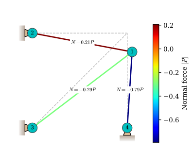
The node moves \(0.79\,PL/EA\) along the load and \(0.21\,PL/EA\) across it, so it does not travel in the direction it is pushed. Of the three rods, only rod 1 ends up in tension; rods 2 and 3 are in compression, with rod 3 carrying by far the most at \(0.79P\). That distribution is worth pausing on, because it is not what a first glance suggests. The load is vertical and rod 3 is the vertical rod, so it takes the largest share, but the diagonal rod still picks up more than a third of it and the horizontal rod is loaded despite being perpendicular to the applied force. Every member participates, because they all share one joint whose displacement they all feel.
When \(\bm A^\mathsf{T}\) is square, the structure is statically determinate and the rod forces follow from the loads alone, \(\bm N = (\bm A^\mathsf{T})^{-1}\bm f\), with no material properties needed. Our \(\bm A^\mathsf{T}\) is \(2 \times 3\), so this truss is statically indeterminate: three unknown rod forces and only two equilibrium equations. The missing information is the deformation relation, exactly as it was for the heated rod of Chapter 8.11. The shape of \(\bm A^\mathsf{T}\) is the count of 8.14.1 in matrix form: one row per free degree of freedom, \(2j - r\), and one column per rod, \(m\), so a square matrix means \(m + r = 2j\).
Seeing the result
Setting \(E = A = L = P = 1\) turns the symbols into numbers we can draw. Figure 8.14.11 puts node 1 where the load takes it, at a quarter of the displacement the numbers give, since a joint that moves most of a rod length is far outside the small movements the method assumes.
Code
num = {E: 1, A: 1, L: 1, P: 1}def numeric(column):"""A symbolic column as plain floats, with every symbol set to one."""return np.array([float(v.subs(num)) for v in column])def result_figure(nodes, elements, presc, U, scale, values, label, fmt, **kwargs):"""The deformed truss coloured by one member quantity, every bar labelled.""" fig, ax = plt.subplots(figsize=(5.8, 4.4)) draw_truss(nodes, elements, presc=presc, displacements=U, scale=scale, values=values, value_label=label, cmap="jet", element_numbers=False, ax=ax, **kwargs) moved = nodes + scale*Ufor k, (i, j) inenumerate(elements): ax.text(*(moved[i-1] + moved[j-1])/2, fmt.format(values[k]), fontsize=8, ha="center", va="center", bbox=dict(boxstyle="square,pad=0.2", facecolor="w", edgecolor="none"))nodes1 = np.array([[1, 1], [0, 1], [0, 0], [1, 0]], dtype=float) # row i is node ielements1 = np.array([[2, 1], [3, 1], [4, 1]]) # rod k runs from node k+1 to node 1presc1 = [3, 4, 5, 6, 7, 8] # nodes 2, 3 and 4 are pinned: both dofs of eachwalls = {2: -90, 3: -90} # two of the pins hang off a wall, not off the groundU1 = np.zeros((4, 2))U1[0] = numeric(u_vec)
Code
fig1 = plt.figure(figsize=(4.2, 5.2))ax1 = fig1.add_axes([0, 0, 1, 0.94]) # the axes fill the frame, the title sits aboveanim1 = animate_truss(nodes1, elements1, U1, presc=presc1, loads=[[1, 0, -1]], support_angles=walls, load_length=0.25, scale_max=0.25, frames=20, ax=ax1, title="deformation scale {scale:.2f}")to_responsive_html(anim1, container_id="truss-ex1-deformation", autoplay=False)
Figure 8.14.11: The truss of Figure 8.14.7 moving under the load, with the displacement growing from nothing to a quarter of the size the numbers give. Node 1 travels in a straight line, down and to the right, and the three pinned nodes stay where they are.
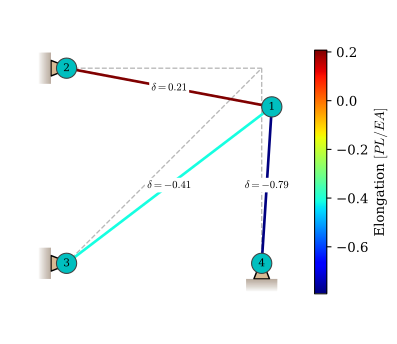
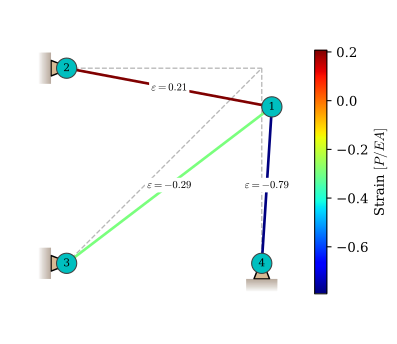
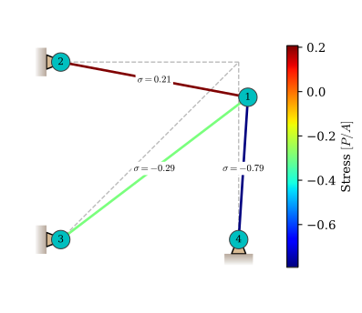
Colouring the same shape by one quantity at a time gives the normal force in Figure 8.14.12, the change in length in Figure 8.14.13, the strain in Figure 8.14.14 and the stress in Figure 8.14.15. Three of the four carry the same colours, because every rod shares one area and one modulus, so \(\sigma_i = N_i/A\) and \(\varepsilon_i = \sigma_i/E\) differ from the force only by a constant. Only the elongation breaks the pattern, and it breaks it at rod 2, the one rod whose length is not \(L\).
Code
result_figure(nodes1, elements1, presc1, U1, 0.25, numeric(N_vec),r"Normal force $[P]$", r"$N={:.2f}P$", support_angles=walls)
Figure 8.14.12: The normal force in each rod, on the deformed shape. Only rod 1 is in tension, and the vertical rod 3 carries most of the load.
Figure 8.14.13: The change in length of each rod. The diagonal rod 2 shortens more than its force alone would suggest, because it is the longest of the three.
Figure 8.14.15: The stress in each rod. With one area shared by all three, this is Figure 8.14.12 in different units.
Example 2: A larger structure
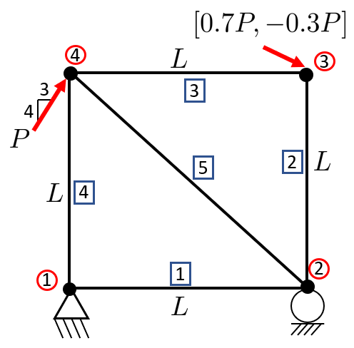
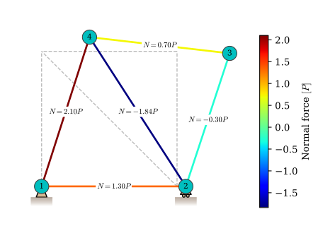
Figure 8.14.16 shows a structure with five rods and four nodes. Node 1 is pinned, so \(u_1^x = u_1^y = 0\), and node 2 rests on a roller, so \(u_2^y = 0\). Node 3 carries the load \([0.7P,\, -0.3P]\), and node 4 carries a load \(P\) with slope \(4/3\), which gives \(f_4^x = \tfrac35 P\) and \(f_4^y = \tfrac45 P\). Rods 1 to 4 have length \(L\), the diagonal rod 5 has length \(\sqrt2 L\), and all five share \(E\) and \(A\).
Figure 8.14.16: A five-rod truss with a pin, a roller and two applied loads.
The method is the one of Example 1, with one change in the bookkeeping. Node 1 is fully fixed and is left out, as the supports were in Example 1. Node 2 is only partly fixed, so we keep both of its degrees of freedom and remove the fixed one after assembly. The displacement and load vectors then have six entries,
where \(f_2^y\) is the unknown reaction from the roller.
Equilibrium of the joints
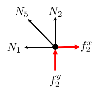
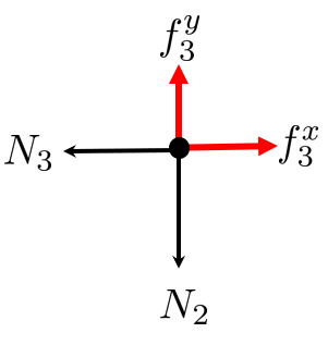
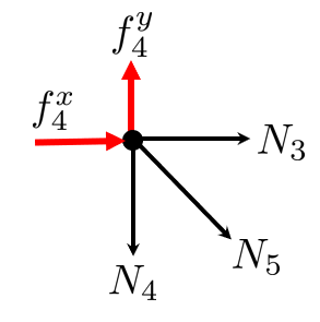
\(\bm A^\mathsf{T}\) has one row for each entry of \(\bm f\) and one column for each rod, so here it is \(6 \times 5\). The rows come from equilibrium of the nodes. We cut each node free as in Figure 8.14.17 to Figure 8.14.19, draw every rod force positive in tension, and balance the forces in \(x\) and in \(y\). Each balance is one row.
Figure 8.14.17: Node 2
Figure 8.14.18: Node 3
Figure 8.14.19: Node 4
A rod in tension pulls a node towards the rod’s far end, and the nodal force \(f_j\) must balance that pull. The coefficient of \(N_i\) in the equation for \(f_j^x\) is therefore the \(x\) component of the unit vector that points along rod \(i\) from its far end towards node \(j\), and likewise for \(y\). A rod that does not touch node \(j\) does not pull on it, and its coefficient is zero.
At node 2, for example, rod 1 comes from node 1 on the left, so its unit vector towards node 2 is \((1, 0)\). Rod 2 comes from node 3 above, giving \((0, -1)\). The diagonal rod 5 comes from node 4 at the top left, giving \((1, -1)/\sqrt2\). Rods 3 and 4 do not reach node 2. Doing the same at nodes 3 and 4, and writing every rod in every equation, including those with coefficient zero, gives
The rows are in the order of \(\bm u\) and \(\bm f\), and within every row the rod forces stand in the same order, \(N_1\) to \(N_5\), each in its own column. The system is already a matrix product. Collecting the coefficients, with their signs, row by row gives \(\bm A^\mathsf{T}\):
Columns 1 and 4 have entries in the rows of one node only, because rods 1 and 4 each have their other end at the fixed node 1, which has no rows. Columns 2, 3 and 5 have entries at both ends of their rod, equal and of opposite sign, since a rod pulls its two nodes towards each other.
The matrix is symmetric, as before, and it is singular: \(\det\bm K = 0\). Without the roller the truss could turn about the pin at node 1 without deforming a single rod, and a structure that can move without deforming has no unique displacement for a given load. The roller is what makes the problem solvable.
Removing the supported degree of freedom
Written out, \(\bm K\bm u = \bm f\) contains the known displacement \(u_2^y = 0\) and, in the same position of the load vector, the unknown reaction \(f_2^y\),
Column 2 multiplies \(u_2^y = 0\) and contributes nothing, and row 2 is the only equation that contains the unknown \(f_2^y\). Deleting both leaves five equations for the five unknown displacements, those of the free degrees of freedom 1, 3, 4, 5 and 6. We number them from one, as in the equations, and let OneArray pick out the rows and columns.
With the displacements known, the rod forces follow from \(\bm N = \bm K^e\bm A\bm u\) as in Example 1, and the full product \(\bm K\bm u\) returns every nodal force, including the reaction \(f_2^y\) that was set aside.
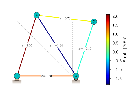
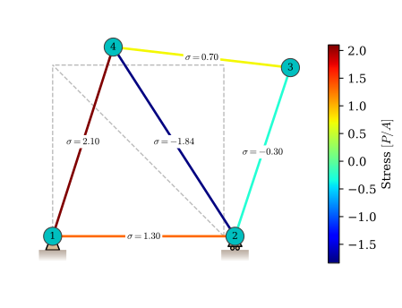
The diagonal rod 5 carries the largest force, \(1.84P\) in compression, and rod 4 the largest tension, \(2.1P\). The roller reaction checks against a moment balance about node 1: the loads at nodes 3 and 4 turn the truss clockwise with \(0.3PL + 0.7PL + 0.6PL = 1.6PL\), and the roller, a distance \(L\) from the pin, answers with \(1.6P\).
Removing the supported degree of freedom also left \(\bm A^\mathsf{T}\) with five rows and five columns. It is square, so by the note in Example 1 this truss is statically determinate, and the rod forces follow from the loads alone, without \(E\), \(A\) or \(L\):
The result is \(\bm N\) again. Setting \(E = A = L = P = 1\) turns this example into numbers too, and Figure 8.14.20 draws the truss where the loads take it. A joint here travels close to eight rod lengths, so the picture is drawn at a twentieth of that, growing from nothing so that the path of each joint can be seen.
Figure 8.14.20: The truss of Figure 8.14.16 moving under its two loads, with the displacement growing from nothing to a twentieth of the size the numbers give. Every joint travels in a straight line, and the pin and the roller hold the two they are attached to.
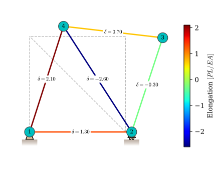
Both top nodes move close to \(8\,PL/EA\) to the right, although no rod changes length by more than \(2.6\,PL/EA\). The square racks: the loads push its top to the right, and only the diagonal rod 5 resists that, by shortening.
The rods in colour
One shape serves four figures: the normal force in Figure 8.14.21, the change in length in Figure 8.14.22, the strain in Figure 8.14.23 and the stress in Figure 8.14.24. The elongations follow from \(\bm\delta = \bm A\bm u\), the strains from \(\varepsilon_i =
\delta_i/L_i\) and the stresses from \(\sigma_i = N_i/A\). Force, stress and strain again differ only by a constant, so only the elongation departs from their pattern, and it departs at the diagonal rod 5.
Figure 8.14.23: The strain in each rod, the elongation divided by the original length. Dividing by the length of rod 5 brings it back into line with the rest.
Figure 8.14.24: The stress in each rod. With one area shared by all five, this is Figure 8.14.21 in different units.
A settling support
Suppose instead that the roller sinks by \(u_2^y = -\tfrac15\,PL/EA\). Column 2 of \(\bm K\) now multiplies a value that is not zero, so it cannot be deleted. Its contribution is known, however, and moves to the right-hand side,
where \(\bm K_{fp}\) is column 2 without its second entry. Figure 8.14.25 shows the two steps: the column is multiplied by the known \(u_2^y\) and carried across to the right-hand side, and only then are row 2 and column 2 struck out. Section 8.15.8 treats the general case.
Figure 8.14.25: Moving the settlement of the roller to the right-hand side before removing its row and column.
\[ \begin{aligned}\bm u_{\text{settled}} - \bm u &=\left[\begin{matrix}0\\- \dfrac{1}{5}\\\dfrac{1}{5}\\- \dfrac{1}{5}\\\dfrac{1}{5}\\0\end{matrix}\right]\frac{PL}{EA}\\ \bm N_{\text{settled}} - \bm N &=\left[\begin{matrix}0\\0\\0\\0\\0\end{matrix}\right]\end{aligned} \]
Not one rod force changes. The extra displacements, \(0.2\,PL/EA\) down at node 2, right and down at node 3 and right at node 4, are those of a rigid rotation about the pin at node 1 by the angle \(P/(5EA)\). A statically determinate truss follows a settling support without resistance, because the loads already fix every rod force through equilibrium. In the statically indeterminate truss of Example 1, moving a support would stretch or compress the rods and load them.
Example 3: Which way should the brace go?
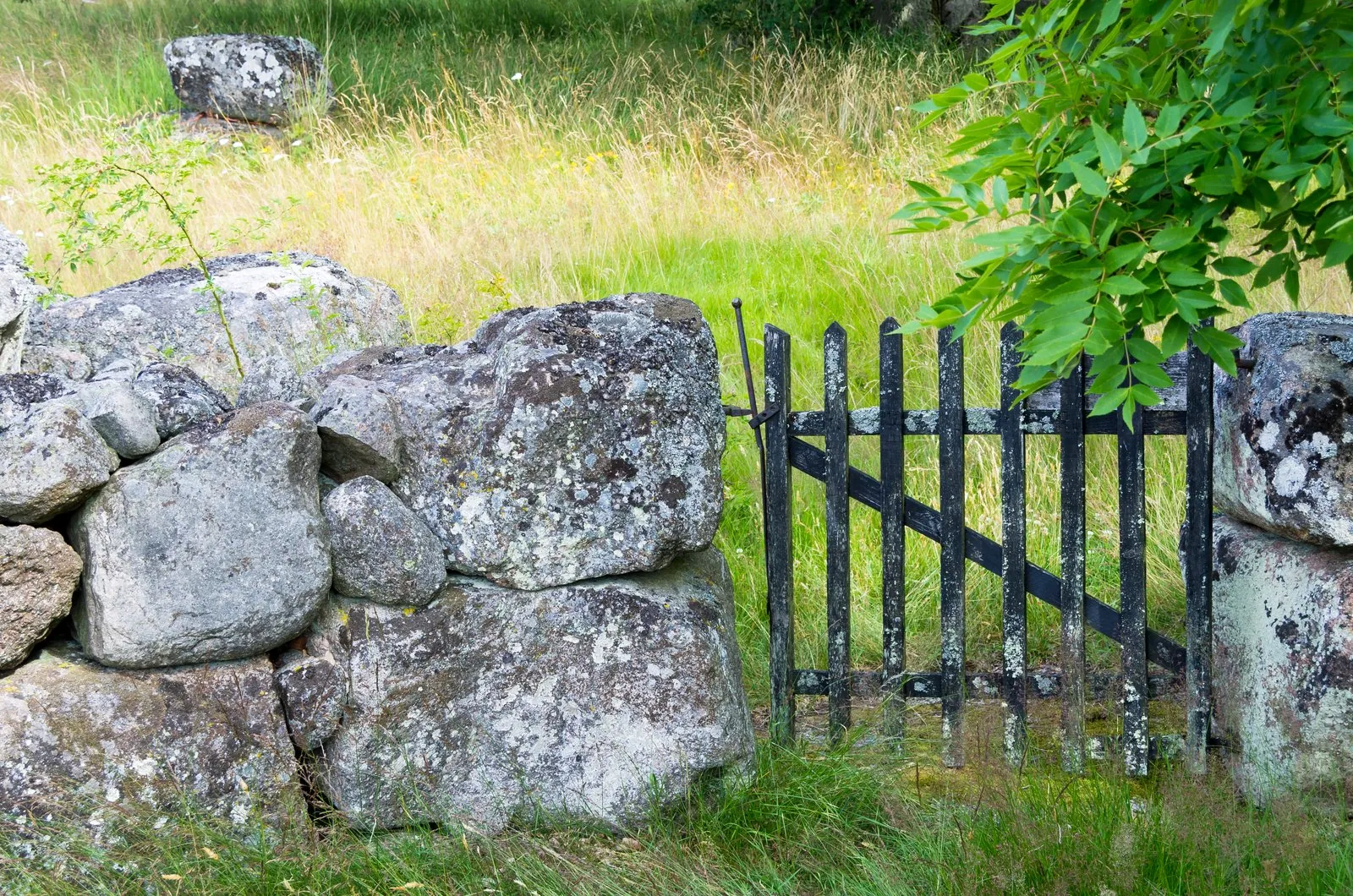
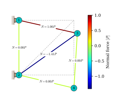
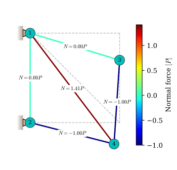
A gate is a truss that everyone has leaned on. Figure 8.14.26 shows one on the island of Tjärö in Blekinge: two rails, two stiles, a row of pickets and a single diagonal brace, hung from two hinges on the post. Its brace drops from the top hinge to the far bottom corner. A carpenter has to choose the direction of that brace, and the two choices in Figure 8.14.27 take the same amount of wood. The question is which one sags less when a load \(P\) hangs on the far top corner, where the latch is and where a child stands to ride the gate open.
Figure 8.14.26: A meadow gate on Tjärö, Blekinge, braced from the top hinge to the far bottom corner.
(a) Design A: the brace runs from the bottom hinge up to the loaded corner.
(b) Design B: the brace runs from the top hinge down to the far bottom corner.
Figure 8.14.27: The two ways to brace a square gate of side \(L\). Every rod shares \(E\) and \(A\), nodes 1 and 2 are the hinges, and the load \(P\) acts at node 3.
The hinges hold nodes 1 and 2 completely. Both are left out as in Example 2, and the free degrees of freedom are those of nodes 3 and 4. Rod 5, the stile between the hinges, has both ends held. Whatever the load, it can neither stretch nor shorten, carries no force, and drops out too. That leaves four rods and four degrees of freedom,
and \(\bm A^\mathsf{T}\) is \(4 \times 4\). Its rows come from the rule of Example 2: the coefficient of \(N_i\) in the row of \(f_j^x\) is the \(x\) component of the unit vector along rod \(i\) from its far end towards node \(j\). The rails and the far stile, rods 1 to 3, are the same in both designs and give the same first three columns. Only the fourth column, the brace, changes. In design A the brace comes into node 3 from node 2, with unit vector \((1, 1)/\sqrt2\) towards node 3, and it appears in the rows of node 3. In design B it comes into node 4 from node 1 with unit vector \((1, -1)/\sqrt2\) and appears in the rows of node 4:
The material matrix is \(EA/L\) times \(\operatorname{diag}(1, 1, 1, 1/\sqrt2)\) for both, so the whole difference between the two gates is one column of \(\bm A^\mathsf{T}\). The code builds the shared columns once and solves both.
frame = sp.Matrix([[1, 0, 0], # f_3^x: rod 1 comes from node 1 on the left [0, 1, 0], # f_3^y: rod 2 comes from node 4 below [0, 0, 1], # f_4^x: rod 3 comes from node 2 on the left [0, -1, 0]]) # f_4^y: rod 2 comes from node 3 abovebrace = {"A": sp.Matrix([s, s, 0, 0]), # into node 3 from node 2, up and right"B": sp.Matrix([0, 0, s, -s])} # into node 4 from node 1, down and rightK_e = (E*A/L) * sp.diag(1, 1, 1, 1/r2)f_gate = sp.Matrix([0, -P, 0, 0])u_gate, N_gate = {}, {}for d in"AB": A_T = frame.row_join(brace[d]) K = sp.simplify(A_T * K_e * A_T.T) u_gate[d] = sp.simplify(K.LUsolve(f_gate)) N_gate[d] = sp.simplify(K_e * A_T.T * u_gate[d])ltx(r"\bm u_A &= \frac{PL}{EA}", sp.simplify(u_gate["A"]/(P*L/(E*A))),r"\approx \frac{PL}{EA}", (u_gate["A"]/(P*L/(E*A))).evalf(3),r",\qquad \bm N_A =", sp.simplify(N_gate["A"]/P), r"P",r"\\\bm u_B &= \frac{PL}{EA}", sp.simplify(u_gate["B"]/(P*L/(E*A))),r"\approx \frac{PL}{EA}", (u_gate["B"]/(P*L/(E*A))).evalf(3),r",\qquad \bm N_B =", sp.simplify(N_gate["B"]/P), r"P", aligned=True)
Both matrices are square, so both gates are statically determinate and the rod forces could have been read from equilibrium alone. Design A puts the brace in compression at \(\sqrt2 P\) and the top rail in tension at \(P\), and leaves the far stile and the bottom rail idle. Design B puts the brace in tension at \(\sqrt2 P\), and now the far stile and the bottom rail each carry \(P\) in compression while the top rail idles. The loaded corner sags \(3.83\,PL/EA\) in design A and \(4.83\,PL/EA\) in design B. The brace that rises from the bottom hinge to the loaded corner gives the stiffer gate, by exactly one \(PL/EA\).
The displacements say where that \(PL/EA\) goes. Node 4 sags \(3.83\,PL/EA\) in both designs. In design A the brace reaches node 3 directly and node 4 hangs below it on an unloaded stile, so the two corners sink together. In design B the load has to travel down the far stile and along the bottom rail before the brace picks it up, and the stile shortens by \(PL/EA\) on the way. That shortening is the extra sag. Figure 8.14.28 draws both gates under the load.
Code
nodes_g = np.array([[0, 1], [0, 0], [1, 1], [1, 0]], dtype=float) # row i is node iframe_rods = [[1, 3], [3, 4], [2, 4]] # rods 1 to 3, the same in both designsbrace_rod = {"A": [2, 3], "B": [1, 4]} # rod 4presc_g = [1, 2, 3, 4] # both hinges hold both of their dofshinges = {1: -90, 2: -90} # and they hang off the post, not the groundfor d in"AB": elements_g = np.array(frame_rods + [brace_rod[d]] + [[1, 2]]) # rod 5 drawn, idle U_g = np.vstack([np.zeros((2, 2)), numeric(u_gate[d]).reshape(2, 2)]) N_g = np.append(numeric(N_gate[d]), 0.0) result_figure(nodes_g, elements_g, presc_g, U_g, 1/16, N_g,r"Normal force $[P]$", r"$N={:.2f}P$", support_angles=hinges)
(a) Design A: the brace pushes, the top rail pulls, and the far stile and bottom rail idle.
(b) Design B: the brace pulls, and the far stile and bottom rail are both compressed by \(P\).
Figure 8.14.28: The two gates under the load, drawn at a sixteenth of the displacement the numbers give and coloured by normal force.
Carpenters brace a wooden gate the way of design A, from the bottom hinge up, and cure a sagging one the way of design B, with a wire and a turnbuckle from the top hinge down. Both habits follow from the forces above. A wooden brace pushes well and pulls badly, since its ends are held by nothing better than nails, and design A is the one that asks it to push. A wire can only pull, and design B is the one that asks it to pull. The Tjärö gate has a wooden brace in the position of the wire: it works in tension, and its nailed joints carry the load.
One thing the model leaves out is buckling. The brace of design A is the longest rod and it is in compression, and a slender member in compression can bow sideways long before its stress reaches anything the material minds. The stiffness comparison stands, but a real brace of design A also needs a check that the rod model cannot make.
Why this is not enough
Everything in this chapter is correct yet none of it scales. The matrix \(\bm A\) was built by inspecting figures, which works for three rods and fails for three hundred. Worse, the construction is tied to this particular set of boundary conditions: fixing a different node changes which degrees of freedom appear in \(\bm u\) and forces the whole matrix to be rebuilt from scratch.
The repair is to stop treating the structure as a whole and start treating each rod as an independent object with its own local coordinate system, expressing its stiffness in that system once and for all and then rotating it into the global frame. Assembling those rotated element matrices into a global system, and only then applying boundary conditions, gives a procedure that a computer can carry out for any truss whatsoever. That is the direct stiffness method, and it is the subject of Chapter 8.15. It is also a window into the finite element method: what changes when we move from trusses to beams, plates and solids is which element matrix goes into the assembly, not the assembly itself.