Code
m, v1, v2, th, dt = 0.43, 15.0, 25.0, np.radians(30), 0.010
J = m*v2*np.array([np.cos(th), np.sin(th)]) - m*np.array([-v1, 0.0])
F_avg = J/dt
J_weight = m*9.81*dt“The Quantity of motion, which is collected by taking the sum of the motions directed towards the same parts, and the difference of those that are directed to contrary parts, suffers no change from the action of bodies among themselves.”
— Isaac Newton, The Mathematical Principles of Natural Philosophy, Corollary III to the Laws of Motion, translated by Andrew Motte, 1729
Work, energy and power integrated Newton’s second law along the path. Integrating it over time instead gives the second great balance of mechanics, between the impulse of the forces and the change of momentum. It answers the questions where forces act for a short time and the time, not the path, is what we know: a kick, a hammer blow, a collision. During an impact the forces are large and unknown, and their history is beyond reach, but their time integral follows from the velocities before and after. The chapter treats the impulse of a single force, the conservation of momentum in a collision, the coefficient of restitution that closes the problem, and the contact model that simulation programs use for the same event.
Newton stated his second law for the linear momentum \(\bm G = m\bm v\), the “quantity of motion” of the epigraph,
\[ \sum\bm F = \frac{d\bm G}{dt} , \]
which for a constant mass is \(\sum\bm F = m\bm a\). Integrating from \(t_1\) to \(t_2\) gives
\[ \bm G_1 + \int_{t_1}^{t_2}\sum\bm F\,dt = \bm G_2 , \qquad \text{i.e.}\qquad m\bm v_1 + \int_{t_1}^{t_2}\sum\bm F\,dt = m\bm v_2 . \tag{7.5.1}\]
The time integral of a force is its impulse, measured in newton seconds. 7.5.1 is a vector equation, one scalar equation per direction. When only the change of velocity and the duration \(\Delta t\) are known, it gives the average force \(\bar{\bm F} = \Delta\bm G/\Delta t\).
The forces of an impact are impulsive: very large and acting for a very short time. Their impulse is finite, of the order of the momentum change. The weight, a spring or a soft support stay of ordinary size, and their impulse during the impact is that ordinary force times \(\Delta t\), which vanishes as \(\Delta t\) does. Over the duration of an impact these non-impulsive forces are left out, and checking that they are small is part of every impact problem.
A football of mass \(m = 0.43\) kg rolls towards the goal line at \(v_1 = 15\) m/s. A defender kicks it away at \(v_2 = 25\) m/s, at the angle \(\theta = 30^\circ\) to the ground (Figure 7.5.1). The foot is in contact with the ball for \(\Delta t = 10\) ms. Find the average force of the kick.
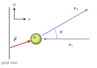
With \(x\) along the ground away from the goal and \(y\) up, the velocities are \(\bm v_1 = [-v_1,\ 0]^\mathsf{T}\) and \(\bm v_2 = v_2[\cos\theta,\ \sin\theta]^\mathsf{T}\). Leaving out the weight for now, 7.5.1 gives the impulse of the kick and its average force,
\[ \bm J = \int_0^{\Delta t}\bm F\,dt = m\bm v_2 - m\bm v_1 , \qquad \bar{\bm F} = \frac{\bm J}{\Delta t} . \]
m, v1, v2, th, dt = 0.43, 15.0, 25.0, np.radians(30), 0.010
J = m*v2*np.array([np.cos(th), np.sin(th)]) - m*np.array([-v1, 0.0])
F_avg = J/dt
J_weight = m*9.81*dtWith the numbers of the example,
\[ {\def\arraystretch{1.3}\begin{aligned}\bm J &=\left[\begin{matrix}15.76\\5.37\end{matrix}\right]~\text{N}\cdot\text{s}, \quad |\bm J| =16.65~\text{N}\cdot\text{s}\\ \bar{\bm F} &=\left[\begin{matrix}1576.0\\537.0\end{matrix}\right]~\text{N}, \quad |\bar{\bm F}| =1665~\text{N} \approx395\,mg\\ mg\,\Delta t &=0.04~\text{N}\cdot\text{s}\end{aligned}} \]
The foot pushes on the ball with 1.67 kN on average, about 400 times the weight of the ball, and mostly along the ground, since most of the momentum change is the reversal of \(v_1\). The impulse of the weight over the 10 ms, 0.04 N·s, is a quarter of a percent of the impulse of the kick, which justifies leaving it out. The force is not constant during the contact: it rises from zero as the ball deforms and falls back to zero as it leaves. For a pulse shaped like half a sine wave the peak is \(\pi/2\) times the average, about 2.6 kN.
For a system of bodies the forces between them come in equal and opposite pairs, and so do their impulses. Summing 7.5.1 over the bodies, the internal impulses cancel, and when the external forces have no impulse, or a negligible one,
\[ \sum_i m_i\bm v_{i1} = \sum_i m_i\bm v_{i2} . \tag{7.5.2}\]
This is the epigraph: the total momentum “suffers no change from the action of bodies among themselves”. In a collision the forces between the bodies are impulsive and the external ones usually are not, so the momentum of the colliding bodies is the same just before and just after the impact, whatever happens during it.
Two bodies moving along one line collide (Figure 7.5.2 shows one case). During the contact they first press into each other until they move with the same velocity, the deformation phase, and then push apart, the restitution phase. Conservation of momentum along the line gives
\[ m_1 v_1 + m_2 v_2 = m_1 v_1' + m_2 v_2' , \]
one equation for the two velocities \(v_1'\) and \(v_2'\) after the impact. The second equation comes from the materials. How much of the deformation is given back is measured by the coefficient of restitution, the ratio of the speed of separation after the impact to the speed of approach before it,
\[ e = \frac{v_2' - v_1'}{v_1 - v_2} , \qquad 0 \leq e \leq 1 . \tag{7.5.3}\]
With \(e = 1\) the impact is perfectly elastic and no kinetic energy is lost; with \(e = 0\) it is perfectly plastic and the bodies move on together. The coefficient depends on the materials, on their shape and on the impact speed, and it is measured, not derived.
m1, m2, u1, u2, e = sp.symbols('m_1 m_2 v_1 v_2 e', real=True)
w1, w2 = sp.symbols("v_1' v_2'", real=True)
sol_c = sp.solve([sp.Eq(m1*u1 + m2*u2, m1*w1 + m2*w2), sp.Eq(w2 - w1, e*(u1 - u2))], [w1, w2], dict=True)[0]
dT = sp.factor(sp.simplify((m1*u1**2 + m2*u2**2 - m1*sol_c[w1]**2 - m2*sol_c[w2]**2)/2))
Solving the two equations, the velocities after the impact and the kinetic energy lost in it are
\[ \begin{aligned}v_1' &=\dfrac{v_{1} \left(- e m_{2} + m_{1}\right) + v_{2} \left(e m_{2} + m_{2}\right)}{m_{1} + m_{2}}\\ v_2' &=\dfrac{v_{1} \left(e m_{1} + m_{1}\right) + v_{2} \left(- e m_{1} + m_{2}\right)}{m_{1} + m_{2}}\\ T - T' &=- \dfrac{m_{1} m_{2} \left(e - 1\right) \left(e + 1\right) \left(v_{1} - v_{2}\right)^{2}}{2 \left(m_{1} + m_{2}\right)}\end{aligned} \]
The energy lost grows with the square of the approach speed and with \(1 - e^2\), and it vanishes only for \(e = 1\).
A steel ball of mass \(m_1 = 0.1\) kg is dropped from the height \(H = 1.0\) m onto a block of mass \(m_2 = 0.5\) kg that rests on a soft foam pad (Figure 7.5.2). The ball rebounds to the height \(h = 0.36\) m. Find the velocity of the block just after the impact, the coefficient of restitution, and the share of the kinetic energy lost.
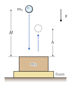
The free fall and the rebound are energy problems of Work, energy and power. With \(y\) positive downwards, the ball arrives with \(v_1 = \sqrt{2gH}\) and leaves upwards with \(v_1' = -\sqrt{2gh}\). The block is at rest, \(v_2 = 0\).
During the impact the foam force and the weights are non-impulsive, so the momentum of ball and block is conserved,
\[ m_1 v_1 = m_1 v_1' + m_2 v_2' \quad\Longrightarrow\quad v_2' = \frac{m_1(v_1 - v_1')}{m_2} , \]
and 7.5.3 and the kinetic energies give
\[ e = \frac{v_2' - v_1'}{v_1} , \qquad \frac{T - T'}{T} = 1 - \frac{m_1 v_1'^2 + m_2 v_2'^2}{m_1 v_1^2} . \]
g = 9.81
m1v, m2v, H, h = 0.1, 0.5, 1.0, 0.36
va = np.sqrt(2*g*H)
va_p = -np.sqrt(2*g*h)
vb_p = m1v*(va - va_p)/m2v
e_drop = (vb_p - va_p)/va
loss = 1 - (m1v*va_p**2 + m2v*vb_p**2)/(m1v*va**2)
With the numbers of the example,
\[ \begin{aligned}v_1 &=4.43~\text{m/s}, \quad v_1' =-2.66~\text{m/s}\\ v_2' &=1.42~\text{m/s}\\ e &=0.92\\ \frac{T - T'}{T} &=12.80~\%\end{aligned} \]
The block is driven into the foam at 1.42 m/s, and the steel-on-steel impact is nearly elastic, \(e = 0.92\), with 13 % of the kinetic energy turned into vibration and heat. The foam then stops the block over a much longer time with a much smaller force, which is what foam packaging is for.
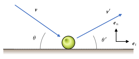
When the velocities are not along the line through the contact, we split them into the component along the common normal \(\bm e_n\) of the contact and the component along the tangent \(\bm e_t\) (Figure 7.5.3). If the surfaces are smooth, the contact force acts along \(\bm e_n\) only, which gives four conditions for two bodies:
For a ball bouncing off a fixed floor the momentum condition drops out, the floor being immovable, and what remains is \(v_t' = v_t\) and \(v_n' = -e\,v_n\). With the angles measured from the floor, \(\tan\theta' = e\tan\theta\): the ball leaves flatter than it arrived, and slower.
The rules of tennis fix the coefficient of restitution of the ball. A ball dropped from 254 cm onto concrete must rebound to more than 135 cm and less than 147 cm (ITF Rules of Tennis, Appendix I). Since the speed at impact is \(\sqrt{2gH}\) and the speed at rebound \(\sqrt{2gh}\), the drop test measures
\[ e = \frac{\sqrt{2gh}}{\sqrt{2gH}} = \sqrt{\frac{h}{H}} , \]
so an approved ball has \(0.728 < e < 0.761\). We take \(e = 0.745\). The ball rolls off a table of height \(h_0 = 0.9\) m with the horizontal speed \(u = 3\) m/s and bounces along a smooth floor. Find its path, the heights of the bounces, and when it stops bouncing.
Between bounces the ball is a projectile, as in Particle kinetics. It lands for the first time after \(t_0 = \sqrt{2h_0/g}\) with the vertical speed \(\sqrt{2gh_0}\). Each bounce keeps the horizontal speed \(u\) and multiplies the vertical speed by \(e\), so the \(n\)-th bounce rises to \(h_n = e^{2n}h_0\) and lasts \(2e^n t_0\) in the air. The times add up to a geometric series,
\[ t_\infty = t_0 + 2t_0\sum_{n=1}^{\infty}e^n = t_0\,\frac{1 + e}{1 - e} , \]
which is finite: after infinitely many ever shorter bounces the ball rolls on at \(u\) after the time \(t_\infty\), having travelled \(u\,t_\infty\).
We integrate the flight with small time steps and apply the bounce rule \(v_y \to -e\,v_y\) whenever the ball reaches the floor moving down, and compare the peaks with \(h_n = e^{2n}h_0\).
def bounce(e=0.745, h0=0.9, u=3.0, g=9.81, T=3.0, dt=1e-5):
    n = int(T/dt)
    x, y, vy = np.zeros(n), np.zeros(n), np.zeros(n)
    y[0] = h0
    for i in range(n - 1):
        vy[i + 1] = vy[i] - g*dt
        y[i + 1] = y[i] + dt*vy[i + 1]
        x[i + 1] = x[i] + dt*u
        if y[i + 1] < 0 and vy[i + 1] < 0:         # the floor: reflect the normal velocity
            y[i + 1], vy[i + 1] = -y[i + 1], -e*vy[i + 1]
    return x, y, vy

e_t, h0, u0 = 0.745, 0.9, 3.0
xb, yb, vyb = bounce(e_t, h0, u0)
t0 = np.sqrt(2*h0/9.81)
t_inf = t0*(1 + e_t)/(1 - e_t)
peaks = np.where((vyb[:-1] > 0) & (vyb[1:] <= 0))[0]
h_sim = yb[peaks][:5]
h_pred = h0*e_t**(2*np.arange(1, 6))fig, ax = plt.subplots(figsize=(6.5, 2.8))
ax.plot(xb, yb, color='C2', lw=1.4)
ax.plot(xb[peaks][:5], h_pred, 'ko', ms=4, label=r'$h_n = e^{2n}h_0$')
ax.axvline(u0*t_inf, color='0.5', ls='--', lw=1)
ax.text(u0*t_inf - 0.1, 0.35, r'$u\,t_\infty$', ha='right')
ax.set_xlabel('$x$ [m]'); ax.set_ylabel('$y$ [m]'); ax.grid(alpha=0.3)
ax.set_xlim(0, 9); ax.set_ylim(0, 0.9); ax.legend(loc='upper center', fontsize=9)
end_ticks(fig)
plt.tight_layout(); plt.show()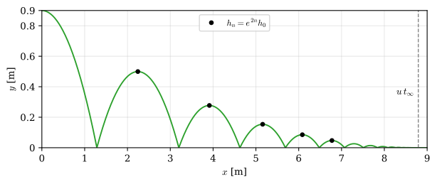
The simulated peaks lie on \(e^{2n}h_0\). The first five bounces, and the time and distance at which the bouncing ends, are
\[ \begin{aligned}h_{1\ldots5}\big|_{\text{simulation}} &=\left[\begin{matrix}0.5 & 0.277 & 0.154 & 0.085 & 0.047\end{matrix}\right]~\text{m}\\ h_{1\ldots5}\big|_{e^{2n}h_0} &=\left[\begin{matrix}0.5 & 0.277 & 0.154 & 0.085 & 0.047\end{matrix}\right]~\text{m}\\ t_\infty &=2.93~\text{s}, \quad u\,t_\infty =8.79~\text{m}\end{aligned} \]
Each bounce keeps \(e^2 = 0.555\) of the vertical kinetic energy, so the peaks fall by almost half each time, and the energy check is built into the comparison: the rebound height is the kinetic energy after the bounce turned back into potential energy. The ball stops bouncing after 2.93 s and 8.8 m. A real tennis ball also picks up spin from friction at each bounce, which the smooth floor of the model leaves out.
The coefficient of restitution describes the impact by its result. A simulation program has to compute what happens during the contact, and the usual model is the one of Figure 7.5.4. While the ball presses into the floor by the penetration \(\delta\), a spring \(k\) and a damper \(c\) push it back; when they are apart, nothing acts. The contact can push but not pull, so the force is
\[ F = \max\bigl(0,\ k\delta + c\dot\delta\bigr) \quad\text{for } \delta > 0 , \qquad F = 0 \quad\text{otherwise} , \]
the force that switches on in the bungee jump of Particle kinetics, with a damper added.
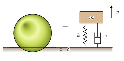
We take the tennis ball of Example 3, of mass \(m = 57\) g and radius 33 mm, and a contact stiffness \(k = 3\cdot 10^4\) N/m, which gives a contact time of a few milliseconds. The damping is then chosen so that the model passes the ITF drop test: dropped from 254 cm, it must come back with \(e = 0.745\). With the height \(y\) of the centre and the penetration \(\delta = R - y\), the equation of motion during the drop is
\[ m\ddot y = -mg + F(\delta, \dot\delta) . \]
We find \(c\) by repeating the drop and adjusting \(c\) until the computed \(e\) is 0.745. Linear vibration theory gives a closed form for a spring and damper that also pull, \(e = \exp\bigl(-\zeta\pi/\sqrt{1 - \zeta^2}\bigr)\) with the damping ratio \(\zeta = c/(2\sqrt{km})\), which we compare with the calibrated model. The energy check is the work-energy theorem over the contact: the change of the ball’s kinetic energy between touching down and lifting off equals the work \(\int F\,\dot y\,dt\) of the contact force, since the weight does no net work between two instants at the same height.
from scipy.optimize import brentq

def drop_test(c, m=0.057, k=3e4, R=0.033, H=2.54, g=9.81, dt=2e-6):
    y, v, t = H + R, 0.0, 0.0
    hist, inside = [], False
    while True:
        delta = R - y
        F = max(k*delta - c*v, 0.0) if delta > 0 else 0.0     # pushes, never pulls
        if delta > 0 and not inside:
            inside, v_in = True, v
        if inside:
            hist.append((t, delta, F, v))
            if delta <= 0:
                h_arr = np.array(hist)
                return -v/v_in, h_arr
        v += dt*(F/m - g)
        y += dt*v
        t += dt

c_cal = brentq(lambda c: drop_test(c)[0] - 0.745, 0.1, 80)
e_cal, hist = drop_test(c_cal)
t_c, d_c, F_c, v_c = hist.T
zeta = c_cal/(2*np.sqrt(3e4*0.057))
e_linear = np.exp(-zeta*np.pi/np.sqrt(1 - zeta**2))
dT_contact = 0.057*(v_c[-1]**2 - v_c[0]**2)/2
W_contact = np.trapezoid(F_c*v_c, t_c)
The calibrated damper, the contact it produces, and the energy check are
\[ \begin{aligned}c &=8.21~\text{N}\cdot\text{s/m}, \quad \zeta =0.099\\ e_{\text{model}} &=0.745, \quad e_{\text{linear}} = e^{-\zeta\pi/\sqrt{1-\zeta^2}} =0.731\\ \text{contact time} &=4.36~\text{ms}, \quad F_{\max} =258~\text{N} \approx461\,mg\\ \Delta T &=-0.6320~\text{J}, \quad \int F\,\dot y\,dt =-0.6341~\text{J}\end{aligned} \]
fig, ax1 = plt.subplots(figsize=(6, 3))
ax1.plot(1e3*(t_c - t_c[0]), F_c, color='C3', lw=2, label='contact force $F$')
ax1.set_xlabel('$t$ [ms]'); ax1.set_ylabel('$F$ [N]'); ax1.grid(alpha=0.3)
ax1.set_xlim(0, 1e3*(t_c[-1] - t_c[0])); ax1.set_ylim(0, 280)
ax2 = ax1.twinx()
ax2.plot(1e3*(t_c - t_c[0]), 1e3*d_c, color='C0', lw=1.5, ls='--', label=r'penetration $\delta$')
ax2.set_ylabel(r'$\delta$ [mm]'); ax2.set_ylim(0, 10)
fig.legend(loc='upper right', bbox_to_anchor=(0.88, 0.93), fontsize=9)
end_ticks(fig)
plt.tight_layout(); plt.show()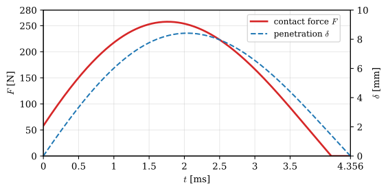
A damping of about ten percent of critical reproduces the tennis ball: contact for 4.4 ms, a peak force of 258 N, more than 450 times the weight, and a rebound to 141 cm, inside the ITF window. The force peaks before the penetration does, because the damper adds to the spring while the ball is still moving in, and it reaches zero while the ball is still slightly pressed in: from then on the spring and the damper would have to pull, which a contact cannot do. That cut-off is why the calibrated model gives \(e = 0.745\) where the linear formula, which lets the damper pull, predicts 0.731. The force also jumps to about 58 N at the instant of touchdown, the damper’s response \(c\dot\delta\) to the impact speed, which a real ball does not show; contact models with a damping term proportional to the penetration, such as the Hunt-Crossley model, remove the jump. The kinetic energy lost in the contact, 0.63 J, equals the work of the contact force to within the accuracy of the time steps.
The rotational counterpart follows from 7.6.2 of Rigid body kinetics, \(\sum M_G = \dot H_G\) with \(H_G = \bar I\omega\). Integrated over time,
\[ \bar I\omega_1 + \int_{t_1}^{t_2}\sum M_G\,dt = \bar I\omega_2 , \]
and the same holds about a fixed pin \(O\) with \(I_O\). The time integral of a moment is its angular impulse. Without an external moment the angular momentum is conserved. A figure skater who pulls in their arms reduces \(\bar I\), and since \(\bar I\omega\) stays the same the skater spins faster.
An impact driver uses angular impulse. Its motor does not turn the bit directly: it spins up a hammer, which strikes an anvil on the bit shaft many times per second. Each blow transfers the hammer’s angular momentum in a fraction of a millisecond, so the moment on the screw during the blow is many times the moment the motor could deliver steadily, while the moment the user’s hand has to hold back is only the small steady moment that spins up the hammer. The energy of each blow is small, but delivered in so short a time it comes out as a large moment, which loosens a screw that a drill of the same power only twists the user’s wrist against.
Meriam, Kraige and Bolton treat impulse, momentum and impact for particles in chapter 3 and for rigid bodies in chapter 6 of their Dynamics [1].