x, L, E, A, F, rho, g = sp.symbols('x L E A F rho g', positive=True)
u = sp.Function('u')

f_body = rho*g*A

ode = sp.Eq(-sp.diff(E*A*sp.diff(u(x), x), x), f_body)
bcs = {u(0): 0, sp.diff(u(x), x).subs(x, L): F/(E*A)}

u_sol = sp.expand(sp.dsolve(ode, u(x), ics=bcs).rhs)8.12 The rod equation
“In itself mathematics is an indivisible organism uniting theoretical contemplation and active application.”
— Richard Courant, Bulletin of the American Mathematical Society, 1943
The Golden Quad of Chapter 8.11, applied to whole bars, produced \(\delta = FL/EA\). That result carries an assumption the geometry hid: the stress is the same everywhere along the bar. Let the cross section taper, or the load act along the length instead of at the end, and there is no single \(N\) to divide by a single \(A\).
The repair is to apply the same three relations to an infinitesimal slice. What comes out is a differential equation with \(\delta = FL/EA\) among its solutions. The reduction runs the other way from Chapter 8.16 here: instead of specialising the continuum we generalise the elementary formula, and the two meet in the middle.
The problem
Figure 8.12.1 shows an elastic rod of constant cross-sectional area \(A\) in \(\text{mm}^2\) hanging from a fixed support. A force \(F\) in \(\text{N}\) acts at the free end \(x = L\), and a body load \(f(x)\) in \(\text{N}/\text{mm}\) acts along its length. Being a force per unit length, \(f\) is where gravity enters.
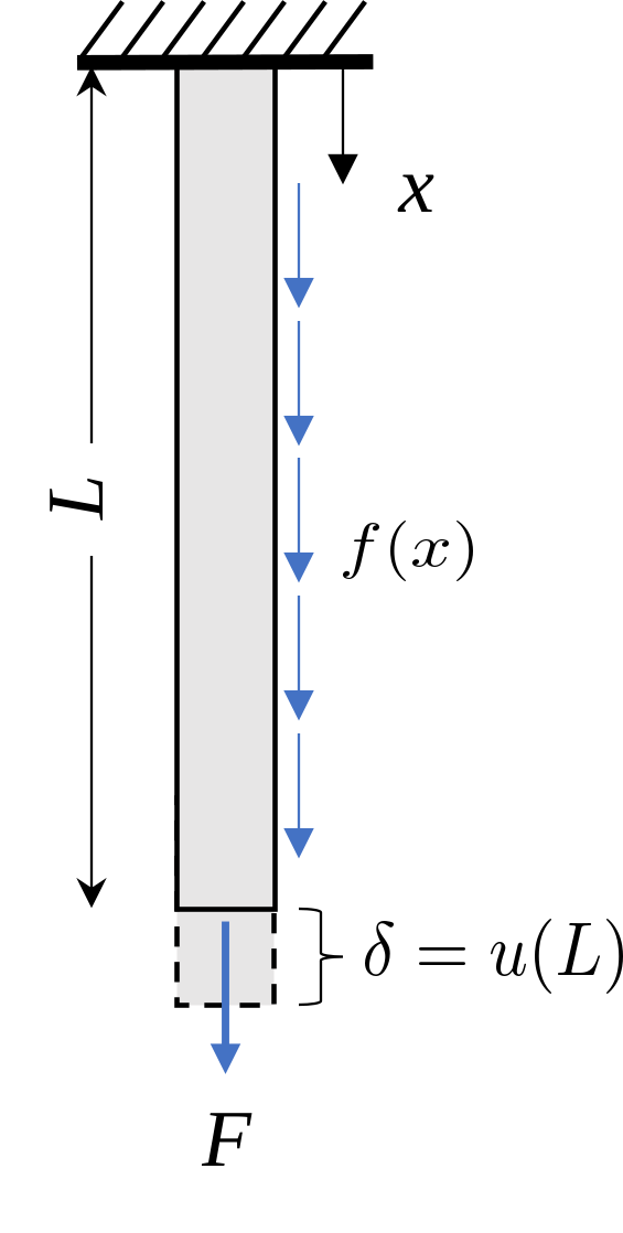
We want \(u(x)\) at every point, given that the rod is fixed at the top, \(u(0) = 0\), and loaded at the bottom by \(F\).
Equilibrium of a slice
Take a slice of length \(\Delta x\) at an arbitrary \(x\), as in Figure 8.12.2. The normal force enters at one end and leaves at the other, and the body load over the slice is the integral of \(f\) across it.
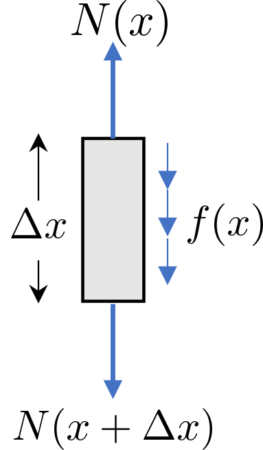
Force equilibrium along the rod gives
\[ N(x + \Delta x) - N(x) + \int_x^{x+\Delta x} f(\xi)\, d\xi = 0 \]
with \(N(L) = F\) at the loaded end. Letting \(\Delta x \to 0\), the integral tends to \(f(x)\Delta x\) and the difference quotient tends to the derivative,
\[ \lim_{\Delta x \to 0} \frac{N(x+\Delta x) - N(x)}{\Delta x} = -f(x) \]
leaving the pointwise equilibrium relation
\[ \boxed{-\frac{dN}{dx} = f} \qquad \text{Equilibrium relation} \tag{8.12.1}\]
This is 8.7.8 integrated over the cross section and written in one dimension. The divergence of the stress has become an ordinary derivative because nothing varies across the section.
The remaining two relations we already have. Forces and stresses are connected by the definition of stress, uniform over the section as always,
\[ \boxed{N = \sigma A} \tag{8.12.2}\]
stresses and strains by Hooke’s law,
\[ \boxed{\sigma = E\varepsilon} \qquad \text{Constitutive relation} \tag{8.12.3}\]
and strains and displacements by 8.5.2. Figure 8.12.3 shows the displacement of each end of the slice; their difference over the slice length is the strain,
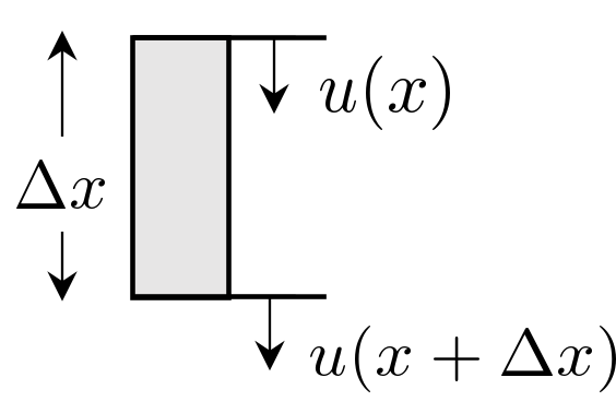
\[ \varepsilon := \lim_{\Delta x \to 0}\frac{u(x+\Delta x) - u(x)}{\Delta x} \;\longrightarrow\; \boxed{\varepsilon = \frac{du}{dx}} \qquad \text{Geometric relation} \tag{8.12.4}\]
The boundary value problem
Substituting 8.12.4 into 8.12.3, the result into 8.12.2 and that into 8.12.1 chains the three relations of the Golden Quad into a single differential equation,
\[ \boxed{ \text{(BVP)}\quad \begin{cases} -\dfrac{d}{dx}\left(EA\dfrac{du}{dx}\right) = f & \text{for } x \in [0, L]\\[10pt] u(0) = 0 & \text{Essential boundary condition}\\[6pt] EA\dfrac{du}{dx}(L) = F & \text{Natural boundary condition} \end{cases}} \tag{8.12.5}\]
Notice that \(EA\) lies inside the derivative. That placement lets the stiffness vary along the rod, and it is why we derive the differential form at all.
The two conditions are of different kinds, and the distinction runs through all of computational mechanics. The condition \(u(0) = 0\) constrains the unknown function itself and is called essential, or Dirichlet. The condition at \(x = L\) constrains \(du/dx\), so through 8.12.2 it prescribes a force, and is called natural, or Neumann. In the finite element method the essential condition must be imposed explicitly on the approximation space, while the natural one appears by itself when the weak form is derived. Hence the name.
⚠ Note
The same pattern reappears in Chapter 8.16. There the fourth-order equation 8.16.13 needs two conditions per end, and 8.16.15 pairs them the same way: prescribing deflection or slope is essential, prescribing moment or shear is natural.
Solving the rod under its own weight
Let the body load be the rod’s own weight, \(f(x) = \rho g A\), with \(\rho\) the density and \(g\) the gravitational acceleration. SymPy solves 8.12.5 directly.
\[ u(x) =\dfrac{L g \rho x}{E} - \dfrac{g \rho x^{2}}{2 E} + \dfrac{F x}{A E} \]
The displacement is quadratic in \(x\): linear from the tip force, quadratic from the weight, since the weight a section carries grows with the rod hanging below it. At the free end it gives the total elongation.
Code
delta = sp.simplify(u_sol.subs(x, L))
ltx(r"\delta = u(L) &=", sp.expand(delta),
    r"\\ \delta\big|_{\rho = 0} &=", sp.expand(delta).subs(rho, 0), aligned=True)
\[ \begin{aligned}\delta = u(L) &=\dfrac{L^{2} g \rho}{2 E} + \dfrac{F L}{A E}\\ \delta\big|_{\rho = 0} &=\dfrac{F L}{A E}\end{aligned} \]
\[ \delta = \frac{FL}{EA} + \frac{\rho g L^2}{2E} \tag{8.12.6}\]
Setting the density to zero recovers \(\delta = FL/EA\): the elementary formula is 8.12.5 with no body load. The self-weight term carries no \(A\), because a thicker rod weighs proportionally more and carries proportionally more, and the two effects cancel. It carries \(L^2\), so it is negligible for a bolt and dominant for a mine hoist rope. Equating the two terms gives the length at which a rod’s own weight matters as much as its payload, \(L = 2F/(\rho g A)\), about \(2.6~\text{km}\) for a steel rod of \(100~\text{mm}^2\) carrying \(10~\text{kN}\).
Code
L_equal = sp.solve(sp.Eq(F*L/(E*A), rho*g*L**2/(2*E)), L)[0]
L_num = L_equal.subs({F: 10e3, rho: 7.85e-6, g: 9.81, A: 100})

ltx(r"L_{\text{equal}} &=", L_equal,
    r"\\ &=", (L_num/1e6).evalf(3), r"~\text{km}", aligned=True)
\[ \begin{aligned}L_{\text{equal}} &=\dfrac{2 F}{A g \rho}\\ &=2.6~\text{km}\end{aligned} \]
A tapered rod
The case that motivated the derivation is a varying \(A\), and it now needs nothing new. Let the rod be conical, tapering linearly from an area \(A_0\) at the support to half that at the tip,
\[ A(x) = A_0\left(1 - \frac{x}{2L}\right) \]
carrying a tip force \(F\) and no body load.
With no body load, 8.12.1 gives \(dN/dx = 0\), so the normal force is constant along the rod and equal to the tip force, \(N = F\). The strain then follows from 8.12.2 and 8.12.3 as \(\varepsilon = F/(EA(x))\), and the displacement is its integral,
\[ u(x) = \int_0^x \frac{F}{EA(\xi)}\,d\xi = -\frac{2FL}{EA_0}\ln\left(1 - \frac{x}{2L}\right), \qquad \delta = u(L) = 2\ln 2\,\frac{FL}{EA_0} \tag{8.12.7}\]
To keep SymPy from picking a branch of the logarithm, we verify this \(u(x)\) against all three parts of 8.12.5.
A_0 = sp.symbols('A_0', positive=True)
A_x = A_0*(1 - x/(2*L))

u_taper = -2*F*L/(E*A_0) * sp.log(1 - x/(2*L))

residual = sp.simplify(-sp.diff(E*A_x*sp.diff(u_taper, x), x))
at_support = u_taper.subs(x, 0)
at_tip = sp.simplify((E*A_x*sp.diff(u_taper, x)).subs(x, L))
\[ \begin{aligned}\text{residual} &=0\\ u(0) &=0\\ \left.EA\dfrac{du}{dx}\right|_{x=L} &=F\end{aligned} \]
Code
delta_taper = sp.simplify(u_taper.subs(x, L))

ltx(r"u(x) &=", u_taper,
    r"\\ \delta &=", delta_taper,
    r"\approx", delta_taper.subs({F: 1, L: 1, E: 1, A_0: 1}).evalf(4), r"\frac{FL}{EA_0}",
    aligned=True)
\[ \begin{aligned}u(x) &=- \dfrac{2 F L \log{\left(1 - \dfrac{x}{2 L} \right)}}{A_{0} E}\\ \delta &=\dfrac{2 F L \log{\left(2 \right)}}{A_{0} E}\approx1.386\frac{FL}{EA_0}\end{aligned} \]
The exact elongation is \(2\ln 2 \approx 1.386\) times \(FL/(EA_0)\). The average area \(\bar A = 0.75 A_0\) gives \(1.333\) times the same quantity, \(4\%\) low. That error stays small while the taper is gentle and grows quickly as the tip narrows: \(1/A(x)\) blows up as the area goes to zero, so a rod tapering to a point has infinite compliance while its average area stays finite.
That is the practical argument for the differential formulation. It asks for one extra line of SymPy and stays right where the algebraic shortcut does not.
The rod as a spring
Setting the body load to zero and holding \(A\) constant reduces 8.12.5 to
\[ \frac{d^2u}{dx^2} = 0 \]
and the two boundary conditions fix the two constants of integration.
u_prism = sp.dsolve(sp.Eq(-sp.diff(E*A*sp.diff(u(x), x), x), 0), u(x),
                    ics={u(0): 0, sp.diff(u(x), x).subs(x, L): F/(E*A)}).rhs
\[ \begin{aligned}u(x) &=\dfrac{F x}{A E}\\ \delta = u(L) &=\dfrac{F L}{A E}\end{aligned} \]
The displacement grows linearly from the support to \(\delta = FL/(EA)\) at the free end, the result Chapter 8.11 reached without calculus in 8.11.5. Read as a force-displacement relation it becomes
\[ F = \frac{EA}{L}\,\delta = k\,\delta, \qquad k = \frac{EA}{L} \tag{8.12.8}\]
so a prismatic rod pulled at its end is a linear spring. The material contributes \(E\), the section \(A\), and the length divides. A steel bar of \(100~\text{mm}^2\) and one metre takes \(21~\text{kN}\) per millimetre of stretch. Torsion gives the same form, \(M = (GJ/L)\,\theta\), by the same route in Chapter 8.13.
Springs compose. Two rods bolted end to end, or thirty pinned into a truss, make a network whose response follows from each member’s stiffness and from the record of which members meet at which joint. Getting from member to network needs no new mechanics, only bookkeeping, and the rest of this chapter sets that bookkeeping up along one axis so Chapter 8.14 can do it in a plane.
A two-node element
Number the ends of a rod 1 and 2, let \(u_1\) and \(u_2\) be their displacements and \(F_1\) and \(F_2\) the forces the surroundings apply there, all positive towards increasing \(x\). A rod treated this way is an element, its ends nodes: the points where elements connect and where the displacement is computed. Each independent nodal displacement, here \(u_1\) and \(u_2\), is a degree of freedom. Figure 8.12.4 draws it as the spring 8.12.8 says it is; Figure 8.12.5 keeps it a rod and adds the free bodies a cut between the nodes produces.
Code
def coil(ax, x0, x1, y=0.0, turns=8, amp=0.26, lead=0.28):
    """A spring drawn between x0 and x1."""
    xa, xb = x0 + lead, x1 - lead
    n = 2*turns
    xs = np.linspace(xa, xb, n + 1)
    ys = np.full(n + 1, float(y))
    ys[1:-1] = y + amp*np.where(np.arange(1, n) % 2 == 1, 1.0, -1.0)
    ax.plot([x0, xa], [y, y], 'k-', lw=1.6, solid_capstyle='round')
    ax.plot(xs, ys, 'k-', lw=1.6, solid_capstyle='round')
    ax.plot([xb, x1], [y, y], 'k-', lw=1.6, solid_capstyle='round')

def node(ax, x, number, y=0.0):
    ax.plot([x], [y], 'o', ms=10, mfc='white', mec='k', mew=1.6, zorder=6)
    ax.text(x, y - 0.78, str(number), ha='center', va='center', fontsize=11, zorder=6,
            bbox=dict(boxstyle='square,pad=0.26', fc='white', ec='k', lw=1))

def element(ax, x0, x1, number, label, y=0.0):
    coil(ax, x0, x1, y)
    ax.text(0.5*(x0 + x1), y + 0.72, label, ha='center', va='center', fontsize=13)
    ax.text(0.5*(x0 + x1), y - 0.78, str(number), ha='center', va='center', fontsize=11,
            zorder=6, bbox=dict(boxstyle='circle,pad=0.24', fc='white', ec='k', lw=1))

def xaxis(ax, x=-0.1, y=-1.55):
    arrow((x, y), (0.8, 0), ax=ax, color='k', linewidth=1.2)
    ax.text(x + 0.85, y, r"$x$", va='center', ha='left', fontsize=12)

fig, ax = plt.subplots(figsize=(6.4, 2.5))
element(ax, 0.0, 3.4, 1, r"$k$")
node(ax, 0.0, 1)
node(ax, 3.4, 2)
arrow((-1.35, 0), (1.0, 0), ax=ax, color=RED)
ax.text(-0.85, 0.30, r"$F_1,\ u_1$", color=RED, ha='center', fontsize=12)
arrow((3.55, 0), (1.0, 0), ax=ax, color=RED)
ax.text(4.05, 0.30, r"$F_2,\ u_2$", color=RED, ha='center', fontsize=12)
xaxis(ax, -1.35)
ax.set_xlim(-1.7, 5.2)
ax.set_ylim(-1.9, 1.2)
ax.set_aspect('equal')
ax.axis('off')
plt.show()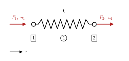
Code
fig, ax = plt.subplots(figsize=(7.0, 4.4))

def bar(x0, x1, y, h=0.16):
    ax.add_patch(plt.Rectangle((x0, y - h), x1 - x0, 2*h,
                               facecolor='#dce6f1', edgecolor='k', lw=1.2, zorder=2))

# the element, its two nodes and the forces the surroundings apply to it
yE = 2.7
bar(0, 4, yE)
ax.plot([0, 4], [yE, yE], 'ko', ms=9, zorder=6)
ax.text(0, yE - 0.52, "1", ha='center', va='center', fontsize=12)
ax.text(4, yE - 0.52, "2", ha='center', va='center', fontsize=12)
arrow((-1.35, yE), (1.0, 0), ax=ax, color=RED)
arrow((4.25, yE), (1.0, 0), ax=ax, color=RED)
ax.text(-0.85, yE + 0.26, r"$F_1,\ u_1$", color=RED, ha='center', fontsize=12)
ax.text(4.75, yE + 0.26, r"$F_2,\ u_2$", color=RED, ha='center', fontsize=12)
ax.plot([2, 2], [yE - 0.55, yE + 0.55], 'k--', lw=1, dashes=(4, 3))
ax.text(2, yE + 0.68, "cut", ha='center', fontsize=11)

# the piece to the left of the cut
yL = 1.3
bar(0, 2, yL)
ax.plot([0], [yL], 'ko', ms=9, zorder=6)
arrow((-1.35, yL), (1.0, 0), ax=ax, color=RED)
ax.text(-0.85, yL + 0.26, r"$F_1$", color=RED, ha='center', fontsize=12)
arrow((2.05, yL), (0.85, 0), ax=ax, color=BLUE)
ax.text(2.48, yL + 0.26, r"$N$", color=BLUE, ha='center', fontsize=12)

# the piece to the right of the cut
yR = 0.0
bar(2, 4, yR)
ax.plot([4], [yR], 'ko', ms=9, zorder=6)
arrow((4.25, yR), (1.0, 0), ax=ax, color=RED)
ax.text(4.75, yR + 0.26, r"$F_2$", color=RED, ha='center', fontsize=12)
arrow((1.95, yR), (-0.85, 0), ax=ax, color=BLUE)
ax.text(1.52, yR + 0.26, r"$N$", color=BLUE, ha='center', fontsize=12)

ax.set_xlim(-2.0, 5.8)
ax.set_ylim(-0.6, 3.7)
ax.set_aspect('equal')
ax.axis('off')
plt.show()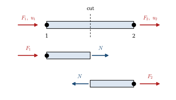
The three relations of Chapter 8.11 are all we need. The elongation is the difference of the end displacements,
\[ \delta = u_2 - u_1 \]
Hooke’s law in the form of 8.12.8 turns that difference into the normal force,
\[ N = k\,(u_2 - u_1) \]
and equilibrium of each free body ties the normal force to the nodal forces. The left piece gives \(F_1 + N = 0\) and the right piece \(F_2 - N = 0\), so \(F_1 = -N\) and \(F_2 = N\), and substituting the normal force,
\[ F_1 = k\,(u_1 - u_2), \qquad F_2 = k\,(u_2 - u_1) \]
Check the signs against the picture. If \(u_2 > u_1\) the rod has been stretched and \(N > 0\). Then \(F_2\) is positive and pulls node 2 towards increasing \(x\), and \(F_1\) is negative and pulls node 1 the other way. They sum to zero: no load acts between the nodes, so \(F_1\) and \(F_2\) are the only forces on the element and static equilibrium balances them.
The two equations are one matrix product,
\[ \underbrace{k\begin{bmatrix} 1 & -1 \\ -1 & 1 \end{bmatrix}}_{\textstyle \bm k^e} \begin{bmatrix} u_1 \\ u_2 \end{bmatrix} = \begin{bmatrix} F_1 \\ F_2 \end{bmatrix} \tag{8.12.9}\]
and \(\bm k^e\) is the element stiffness matrix of a rod. Column \(j\) holds the nodal forces that keep the element in the state where node \(j\) has moved one unit and the other has not. Chapter 8.14 applies that same unit displacement construction to a truss. The matrix is symmetric, and so is everything assembled from it. Its rows sum to zero, so translating both nodes together produces no forces and the matrix is singular: an element on its own floats, and 8.12.9 cannot be solved until something holds it.
Assembling a chain
Two rods joined end to end are enough to show what assembly does. Figure 8.12.6 numbers the nodes 1, 2 and 3 from left to right, so element 1 spans nodes 1 and 2 with stiffness \(k_1\), element 2 nodes 2 and 3 with \(k_2\). The record of which nodes each element connects is the topology, and with the two stiffnesses it is everything the assembly needs. A structure divided into elements that share nodes is a mesh, and the topology is its description.
Code
X = [0.0, 2.9, 5.8]
fig, ax = plt.subplots(figsize=(6.8, 2.5))

for e, (a, b) in enumerate(zip(X[:-1], X[1:]), start=1):
    element(ax, a, b, e, rf"$k_{e}$")
for m, xm in enumerate(X, start=1):
    node(ax, xm, m)
    ax.text(xm, 0.72, rf"$F_{m},\ u_{m}$", ha='center', va='center',
            fontsize=12, color=RED)
xaxis(ax)

ax.set_xlim(-0.75, 6.55)
ax.set_ylim(-1.9, 1.2)
ax.set_aspect('equal')
ax.axis('off')
plt.show()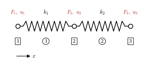
Three nodal displacements and three nodal forces make a three by three system. Each element contributes to the rows and columns of its own nodes and nowhere else, so element 1 reaches 1 and 2 while element 2 reaches 2 and 3, as Figure 8.12.7 shows. Written at the size of the structure, with zeros where an element does not reach, the two contributions add.
Code
E1_c, E2_c, F1_c, F2_c = '#b22222', '#1f4e79', '#f2dede', '#dce6f1'

def matrix_grid(ax, labels, entries, boxes, title):
    m = len(labels)
    for r in range(m):
        for c in range(m):
            ax.add_patch(plt.Rectangle((c, -r), 1, -1, lw=0.7,
                                       facecolor=entries[r][c][1], edgecolor='0.75'))
            ax.text(c + 0.5, -r - 0.5, entries[r][c][0], ha='center', va='center', fontsize=11)
    for q, lab in enumerate(labels):
        ax.text(q + 0.5, 0.34, lab, ha='center', va='center', fontsize=11)
        ax.text(-0.34, -q - 0.5, lab, ha='center', va='center', fontsize=11)
    for lo, hi, colour, inset in boxes:
        side = (hi - lo + 1) - 2*inset
        ax.add_patch(plt.Rectangle((lo + inset, -lo - inset), side, -side, lw=2.0,
                                   facecolor='none', edgecolor=colour, zorder=5))
    ax.set_title(title, fontsize=11, pad=9)
    ax.set_xlim(-0.85, m + 0.15)
    ax.set_ylim(-m - 0.15, 0.85)
    ax.set_aspect('equal')
    ax.axis('off')

fig, axes = plt.subplots(1, 3, figsize=(10.5, 3.3),
                         gridspec_kw={'width_ratios': [1, 1, 1.45]})
matrix_grid(axes[0], ["1", "2"],
            [[(r"$k_1$", F1_c), (r"$-k_1$", F1_c)],
             [(r"$-k_1$", F1_c), (r"$k_1$", F1_c)]],
            [(0, 1, E1_c, 0.03)], "element 1, nodes 1 and 2")
matrix_grid(axes[1], ["2", "3"],
            [[(r"$k_2$", F2_c), (r"$-k_2$", F2_c)],
             [(r"$-k_2$", F2_c), (r"$k_2$", F2_c)]],
            [(0, 1, E2_c, 0.03)], "element 2, nodes 2 and 3")
matrix_grid(axes[2], ["1", "2", "3"],
            [[(r"$k_1$", F1_c),  (r"$-k_1$", F1_c),             ("0", 'white')],
             [(r"$-k_1$", F1_c), (r"$k_1\!+\!k_2$", '#e2dfea'), (r"$-k_2$", F2_c)],
             [("0", 'white'),    (r"$-k_2$", F2_c),             (r"$k_2$", F2_c)]],
            [(0, 1, E1_c, 0.03), (1, 2, E2_c, 0.11)], r"structure matrix $\mathbf{K}$")
plt.show()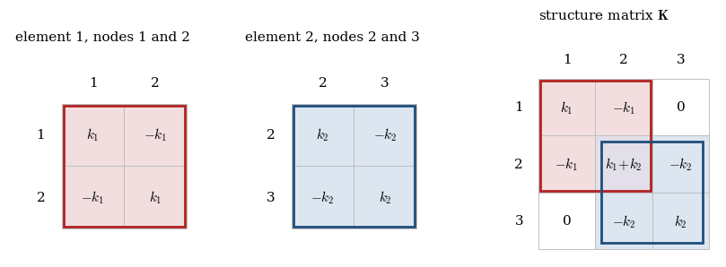
k_1, k_2 = sp.symbols('k_1 k_2', positive=True)
k_rod = sp.Matrix([[1, -1], [-1, 1]])

K_e1, K_e2 = sp.zeros(3, 3), sp.zeros(3, 3)
K_e1[0:2, 0:2] = k_1*k_rod
K_e2[1:3, 1:3] = k_2*k_rod
\[ \begin{aligned}\bm K^{e_1} &=\left[\begin{matrix}k_{1} & - k_{1} & 0\\- k_{1} & k_{1} & 0\\0 & 0 & 0\end{matrix}\right], \quad \bm K^{e_2} =\left[\begin{matrix}0 & 0 & 0\\0 & k_{2} & - k_{2}\\0 & - k_{2} & k_{2}\end{matrix}\right]\\ \bm K &=\left[\begin{matrix}k_{1} & - k_{1} & 0\\- k_{1} & k_{1} + k_{2} & - k_{2}\\0 & - k_{2} & k_{2}\end{matrix}\right]\end{aligned} \]
Node 2 belongs to both rods, so its diagonal entry collects a contribution from each and the joint comes out stiffer than either rod alone. The corner entries stay at zero because nodes 1 and 3 are not connected directly, and a displacement at one reaches the other only through node 2.
Full-size matrices are almost all zeros once a structure has more than a few nodes, and no code builds them. What the code keeps is the two by two element matrix, added into the rows and columns its nodes occupy. For an element spanning global nodes \(i\) and \(j\),
\[ \bm K([i,j],[i,j]) \mathrel{{+}{=}} \bm k^e \tag{8.12.10}\]
which in Python is the same line, K[[i, j], [i, j]] += ke, once K is a MechanicsKit OneArray and \(i\) and \(j\) are the node numbers of Figure 8.12.6. NumPy would want K[np.ix_([i-1, j-1], [i-1, j-1])], and each of those subtractions is a chance to write a bug that reads like a modelling error. The += makes this assembly instead of assignment: a shared node is written to more than once and every visit adds to what is there. Figure 8.12.8 follows four elements of a five-node chain into the structure matrix, shading each entry by the number of elements that have reached it.
Code
n = 5
shades = ['white', '#cfe0f2', '#7fa8d4']
fig, axes = plt.subplots(1, n - 1, figsize=(10.5, 3.2))
hits = OneArray(np.zeros((n, n), dtype=int))

for e, ax in enumerate(axes, start=1):
    i, j = e, e + 1                          # the two nodes of element e
    hits[[i, j], [i, j]] += 1
    for r in range(1, n + 1):
        for c in range(1, n + 1):
            ax.add_patch(plt.Rectangle((c - 1, 1 - r), 1, -1, lw=0.7,
                                       facecolor=shades[min(hits[r, c], 2)],
                                       edgecolor='0.7'))
    ax.add_patch(plt.Rectangle((i - 1, 1 - i), 2, -2, lw=2.0,
                               facecolor='none', edgecolor='#b22222', zorder=5))
    for m in range(1, n + 1):
        ax.text(m - 0.5, 0.35, str(m), ha='center', va='center', fontsize=10)
        ax.text(-0.35, 0.5 - m, str(m), ha='center', va='center', fontsize=10)
    ax.set_title(rf"element {e}:  $\mathbf{{K}}([{i},{j}],[{i},{j}])$",
                 fontsize=11, pad=10)
    ax.set_xlim(-0.9, n + 0.2)
    ax.set_ylim(-n - 0.2, 0.9)
    ax.set_aspect('equal')
    ax.axis('off')

plt.show()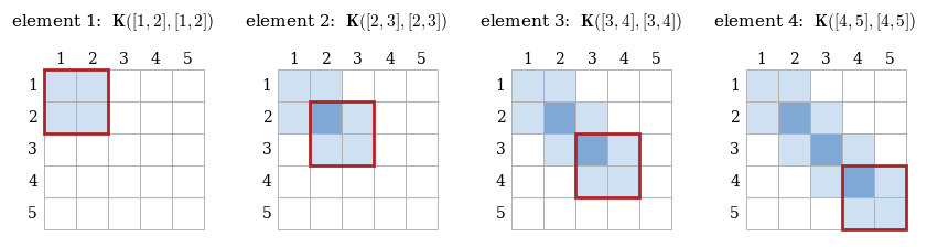
Known and unknown
The assembled matrix is singular for the reason the element matrix was: nothing holds the chain, and adding the same displacement to every node changes no force. Supports remove that freedom, and the rule for applying them is the accounting rule of the method: every degree of freedom carries exactly one known quantity. Either its displacement is prescribed and the force there is an unknown reaction, or the force is prescribed, possibly as zero, and the displacement is unknown. Never both, and never neither.
Sorting the degrees of freedom into a free set \(f\) and a prescribed set \(p\) splits the system into the four blocks of Figure 8.12.9.
Code
FREE_c, PRESC_c = '#cfe0f2', '#f6dcdc'
fig, ax = plt.subplots(figsize=(8.6, 3.4))

def blk(x0, y0, w, h, fc, lab, fs=13):
    ax.add_patch(plt.Rectangle((x0, y0), w, h, facecolor=fc, edgecolor='k', lw=1.2))
    ax.text(x0 + w/2, y0 + h/2, lab, ha='center', va='center', fontsize=fs)

a, b = 1.9, 1.1                       # size of the free and the prescribed blocks
blk(0, b, a, a, FREE_c,  r"$\mathbf{K}_{ff}$")
blk(a, b, b, a, PRESC_c, r"$\mathbf{K}_{fp}$")
blk(0, 0, a, b, FREE_c,  r"$\mathbf{K}_{pf}$")
blk(a, 0, b, b, PRESC_c, r"$\mathbf{K}_{pp}$")

xu = a + b + 0.35
blk(xu, b, 0.62, a, FREE_c,  r"$\mathbf{u}_f$", 12)
blk(xu, 0, 0.62, b, PRESC_c, r"$\mathbf{u}_p$", 12)
ax.text(xu + 0.98, (a + b)/2, "=", ha='center', va='center', fontsize=18)
xf = xu + 1.35
blk(xf, b, 0.62, a, FREE_c,  r"$\mathbf{f}_f$", 12)
blk(xf, 0, 0.62, b, PRESC_c, r"$\mathbf{f}_p$", 12)

ax.text(-0.22, b + a/2, "free", ha='right', va='center', fontsize=11, color='#1f4e79')
ax.text(-0.22, b/2, "prescribed", ha='right', va='center', fontsize=11, color='#b22222')
ax.text(a/2, a + b + 0.2, "free", ha='center', fontsize=11, color='#1f4e79')
ax.text(a + b/2, a + b + 0.2, "prescribed", ha='center', fontsize=11, color='#b22222')

ax.annotate('', xy=(xf + 0.31, b + a + 0.12), xytext=(a + b/2, b + a + 0.12),
            arrowprops=dict(arrowstyle='-|>', color='#b22222', lw=1.6,
                            connectionstyle="arc3,rad=-0.38"))
ax.text((a + b/2 + xf)/2 + 0.1, b + a + 1.0,
        r"known, so it moves across as $-\mathbf{K}_{fp}\mathbf{u}_p$",
        ha='center', fontsize=11, color='#b22222')

ax.set_xlim(-1.6, xf + 1.0)
ax.set_ylim(-0.4, b + a + 1.5)
ax.set_aspect('equal')
ax.axis('off')
plt.show()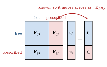
The upper row of that system contains known loads and unknown displacements only,
\[ \boxed{\bm K_{ff}\,\bm u_f = \bm f_f - \bm K_{fp}\,\bm u_p} \tag{8.12.11}\]
and is the system we solve. A prescribed displacement multiplies its own column of \(\bm K\) and crosses to the right-hand side, where it acts as the load that would have produced the same movement. When every prescribed displacement is zero the subtraction vanishes and the reduction is nothing more than striking out rows and columns. Once \(\bm u_f\) is known, the lower row returns the reactions,
\[ \bm f_p = \bm K_{pf}\,\bm u_f + \bm K_{pp}\,\bm u_p \]
\(\bm K_{ff}\) is invertible as soon as the supports remove every rigid body motion, which along one axis means holding at least one node. Chapter 8.15 uses 8.12.11 unchanged, with two displacement components per node instead of one.
Example 1: A chain held at both ends
Two steel rods of area \(A = 100~\text{mm}^2\) meet at node 2, with \(L_1 = 2000~\text{mm}\), \(L_2 = 1400~\text{mm}\) and \(E = 210~\text{GPa}\). Node 1 is fixed, a load \(P = 10~\text{kN}\) pulls node 2 towards the far support, and node 3 is pushed back towards the first rod by \(\delta = 0.5~\text{mm}\).
Code
X = [0.0, 3.2, 5.44]
fig, ax = plt.subplots(figsize=(7.4, 2.6))

def wall(x_w, side):
    ax.add_patch(plt.Rectangle((x_w, -0.62), side*0.20, 1.24, facecolor='none',
                               edgecolor='k', hatch='///', lw=1.0))
    ax.plot([x_w, x_w], [-0.62, 0.62], 'k-', lw=1.6)

for a, b, shade in ((X[0], X[1], '#dce6f1'), (X[1], X[2], '#c3d6ea')):
    ax.add_patch(plt.Rectangle((a, -0.20), b - a, 0.40, facecolor=shade,
                               edgecolor='k', lw=1.2, zorder=2))
wall(X[0], -1)
wall(X[2], +1)
ax.plot(X, [0, 0, 0], 'ko', ms=9, zorder=6)

for m, xm in enumerate(X, start=1):          # nodes in squares
    ax.text(xm, 0.80, str(m), ha='center', va='center', fontsize=11,
            bbox=dict(boxstyle='square,pad=0.26', fc='white', ec='k', lw=1))
for e, (a, b) in enumerate(zip(X[:-1], X[1:]), start=1):   # elements in circles
    ax.text(0.5*(a + b), -0.80, str(e), ha='center', va='center', fontsize=11,
            bbox=dict(boxstyle='circle,pad=0.24', fc='white', ec='k', lw=1))

arrow((X[1], 0.0), (1.0, 0), ax=ax, color=RED, zorder=8)
ax.text(X[1] + 0.5, 0.26, r"$P$", color=RED, ha='center', fontsize=12)
arrow((X[2] + 1.55, 0.0), (-1.0, 0), ax=ax, color=BLUE)
ax.text(X[2] + 1.05, 0.28, r"$u_3 = -\delta$", color=BLUE, ha='center', fontsize=12)

ax.annotate('', xy=(X[0], 1.80), xytext=(X[1], 1.80),
            arrowprops=dict(arrowstyle='<->', lw=1))
ax.annotate('', xy=(X[1], 1.80), xytext=(X[2], 1.80),
            arrowprops=dict(arrowstyle='<->', lw=1))
ax.text(0.5*(X[0] + X[1]), 1.97, r"$L_1,\ A,\ E$", ha='center', fontsize=11)
ax.text(0.5*(X[1] + X[2]), 1.97, r"$L_2,\ A,\ E$", ha='center', fontsize=11)

arrow((-0.15, -1.55), (0.9, 0), ax=ax, color='k', linewidth=1.2)
ax.text(0.9, -1.55, r"$x$", va='center', ha='left', fontsize=12)

ax.set_xlim(-0.6, 7.2)
ax.set_ylim(-1.9, 2.5)
ax.set_aspect('equal')
ax.axis('off')
plt.show()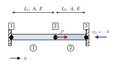
The stiffnesses follow from 8.12.8, and the assembly is the loop of 8.12.10 written out for two elements.
E_num, A_num = 210e3, 100.0                     # MPa, mm^2
L_e = OneArray([2000.0, 1400.0])                # mm, element 1 and element 2
k_e = E_num*A_num/L_e                           # N/mm, one stiffness per element
elements = OneArray([[1, 2], [2, 3]])           # the nodes each element connects
k_rod = np.array([[1.0, -1.0], [-1.0, 1.0]])

K = OneArray(np.zeros((3, 3)))
for e, (i, j) in enumerate(elements, start=1):
    K[[i, j], [i, j]] += k_e[e]*k_rod
\[ \begin{aligned}\begin{bmatrix} k_1 \\ k_2 \end{bmatrix} &=\begin{bmatrix}10500 \\ 15000\end{bmatrix}~\text{N}/\text{mm}\\ \bm K &=\begin{bmatrix}10500 & -10500 & 0 \\ -10500 & 25500 & -15000 \\ 0 & -15000 & 15000\end{bmatrix}~\text{N}/\text{mm}\end{aligned} \]
Nodes 1 and 3 carry prescribed displacements and unknown reactions; node 2 carries the known load \(P\) and an unknown displacement. That is the split 8.12.11 asks for, and here it leaves a single equation.
P, delta = 10e3, 0.5                            # N, mm
uu, ff = OneArray(np.zeros(3)), OneArray(np.zeros(3))

presc, free = [1, 3], [2]                       # node numbers, not array positions
uu[presc] = [0.0, -delta]
ff[free] = P

uu[free] = np.linalg.solve(K[free, free],
                           ff[free] - K[free, presc] @ uu[presc])
ff = K @ uu                                     # all nodal forces, reactions included
\[ \begin{aligned}\bm u &=\begin{bmatrix}0.000 \\ 0.098 \\ -0.500\end{bmatrix}~\text{mm}\\ \bm f &=\begin{bmatrix}-1.029 \\ 10.000 \\ -8.971\end{bmatrix}~\text{kN}\end{aligned} \]
Node 2 ends up \(0.098~\text{mm}\) from where it started: the load pulls it one way, the half millimetre imposed at node 3 pulls it the other, and the two nearly cancel. The reactions come out at \(-1.03~\text{kN}\) at the support and \(-8.97~\text{kN}\) at the pushed node, and the three nodal forces sum to zero, global equilibrium and the fastest check on the arithmetic.
The normal force in each element comes from the same relation that built the element matrix, and the stress from the definition 8.12.2.
NN = OneArray([k_e[e]*(uu[j] - uu[i])
               for e, (i, j) in enumerate(elements, start=1)])
\[ \begin{aligned}\bm N &=\begin{bmatrix}1.029 \\ -8.971\end{bmatrix}~\text{kN}\\ \bm \sigma &=\begin{bmatrix}10.294 \\ -89.706\end{bmatrix}~\text{MPa}\\ \textstyle\sum_i f_i &=0.000~\text{kN}\end{aligned} \]
The first rod is in tension at \(10.3~\text{MPa}\), the second in compression at \(-89.7~\text{MPa}\), both far inside what steel tolerates. The normal forces differ by the \(10~\text{kN}\) applied at node 2, as equilibrium of that joint requires, and they carry opposite signs because the imposed displacement pushes harder than the load pulls. Prescribing a displacement is a stiff way to load a structure: the force it produces is whatever the structure’s own stiffness demands.
Example 2: The same chain with a free end
Releasing node 3 of Example 1 and applying \(P = 20~\text{kN}\) there leaves node 1 as the only support, Figure 8.12.11.
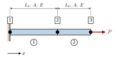
Nothing in the procedure changes apart from which degrees of freedom belong to which set.
uu_2, ff_2 = OneArray(np.zeros(3)), OneArray(np.zeros(3))

presc_2, free_2 = [1], [2, 3]
ff_2[3] = 20e3

uu_2[free_2] = np.linalg.solve(K[free_2, free_2],
                               ff_2[free_2] - K[free_2, presc_2] @ uu_2[presc_2])
ff_2 = K @ uu_2
\[ \begin{aligned}\bm u &=\begin{bmatrix}0.000 \\ 1.905 \\ 3.238\end{bmatrix}~\text{mm}\\ \bm f &=\begin{bmatrix}-20.000 \\ 0.000 \\ 20.000\end{bmatrix}~\text{kN}\\ \delta_{\text{series}} &=3.238~\text{mm}\end{aligned} \]
Both rods carry the full \(20~\text{kN}\), the reaction at node 1 balances it, and node 3 moves by the sum of the two elongations. The last line evaluates that sum from 8.11.6 and matches the assembled answer to the last digit. The bookkeeping reproduces the series rule of Chapter 8.11 without being told it, because the rule was never a separate fact, only a consequence of every joint being in equilibrium and every rod obeying 8.12.8.
What we have and what is missing
8.12.5 is a complete model of an axially loaded member, and it has the same structure as every field problem in this book: a differential equation from equilibrium, a constitutive law inside it, and two boundary conditions of different kinds. Replacing \(EA\) by a thermal conductivity, \(u\) by a temperature and \(f\) by heat generation turns it into steady heat conduction without changing a symbol of the mathematics, and one finite element code therefore solves both.
A chain of rod elements is a straight truss. Its assembly rule 8.12.10, its accounting of knowns against unknowns and its reduction 8.12.11 all carry over untouched to members pointing in different directions. 8.12.9 does not: a rod at an angle moves its nodes in two directions at once, and its two by two matrix has to be rotated into the frame the structure is measured in. That rotation, and the four by four element matrix it produces, is the subject of Chapter 8.14 and Chapter 8.15.