9.4  A printed ball bearing on steel balls

Rolling bearings are the machine element a course normally tells students to buy rather than design, and inside the range a catalogue covers the advice is sound: a 6804 costs a few euro and arrives the next day. It weakens at large diameters, where the price of a thin section bearing climbs steeply with bore, and it fails outright on the afternoon a prototype has to turn.

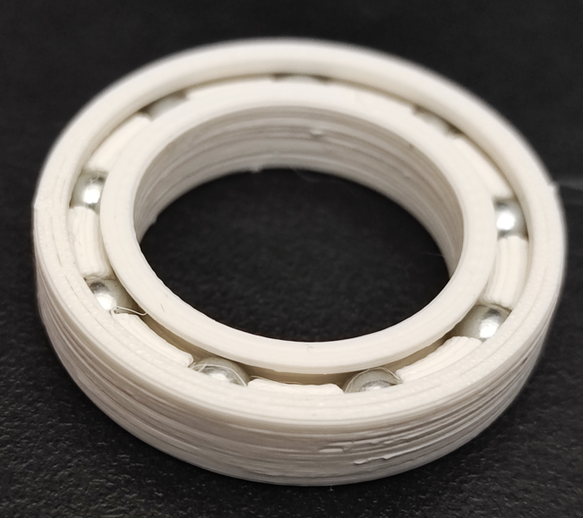
What follows is a working substitute. The rolling elements are 4.5 mm steel airsoft balls, which cost almost nothing and are far rounder than anything they will run against, and the four parts around them are printed: an inner ring, an outer ring, a cap that closes the outer race, and a cage. Figure 9.4.1 shows two finished units. The envelope is that of a 6804, a 20 mm bore with a 32 mm outside diameter and a 7 mm width [1], so a printed bearing drops into a housing dimensioned for the bought one and can be swapped for it later.

Figure 9.4.1: Two finished bearings on the 6804 envelope, printed in PLA and running on nine 4.5 mm steel balls. The layer lines across the bore and the outside surface are the as printed finish. The surfaces that carry load are the races hidden inside, and they are printed to the same standard.

The rolling element

Steel balls sold by the bottle as 4.5 mm air pistol ammunition are the cheapest precision spheres available, and their size is what makes them useful here. A 4.5 mm ball sits inside the 6 mm radial section of a 6804 and still leaves enough plastic on either side to print, which is the constraint that decides the rest of the design. Figure 9.4.2 shows the source.

Figure 9.4.2: The rolling elements: 4.5 mm steel balls sold for air pistols. The packaging states the calibre and nothing about grade or sphericity, which is tolerable here because the printed races are by a wide margin the rougher of the two surfaces in contact.

Fitting the balls into the envelope

Placing the ball centres on the mid-radius of the section,

\[ r_m = \frac{d + D}{4} \]

puts them 13 mm from the axis and leaves the same thickness of material inside and outside. The radial section \((D - d)/2\) measures 6 mm, of which the ball takes 4.5 mm, so 1.5 mm is left to divide between two race walls and two running clearances.

The race groove is an arc of radius

\[ r_g = \frac{d_w}{2} + c \]

struck about the ball centre, with \(c\) the radial clearance between ball and race. Setting \(c\) to 0.05 mm fixes everything else.

Code
import numpy as np
from mechanicskit import ltx

d, D, B = 20.0, 32.0, 7.0        # bore, outside diameter, width of a 6804
d_w, c = 4.5, 0.05               # ball diameter and radial race clearance

r_m = (d + D) / 4                # ball centre radius
r_g = d_w / 2 + c                # race groove radius
t_o = D / 2 - (r_m + r_g)        # wall outside the groove
t_i = (r_m - r_g) - d / 2        # wall inside the groove
f = r_g / d_w                    # race conformity

ltx(r"r_m &=", r_m, r"\ \text{mm}",
    r"\\ r_g &=", r_g, r"\ \text{mm}",
    r"\\ t_\mathrm{o} = t_\mathrm{i} &=", t_o, r"\ \text{mm}",
    r"\\ f &=", f, aligned=True, precision=3)

\[ \begin{aligned}r_m &=13.000\ \text{mm}\\ r_g &=2.300\ \text{mm}\\ t_\mathrm{o} = t_\mathrm{i} &=0.700\ \text{mm}\\ f &=0.511\end{aligned} \]

Both walls come out at 0.70 mm, which is two perimeters at a 0.35 mm extrusion width and the thinnest section anywhere in the bearing. The conformity \(f = r_g / d_w\) lands on 0.511, a little below the 0.515 to 0.53 that catalogue deep groove bearings use [2]. A groove that conforms more closely to the ball spreads the contact over a larger area and lowers the pressure the plastic sees, at the price of more sliding within the contact patch, and for a race that is weak and turns slowly that is the right direction to err in. The value was not aimed at: it follows from rounding the clearance to 0.05 mm.

How many balls

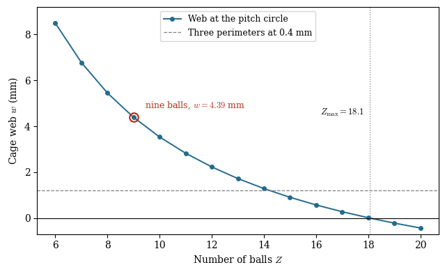
Balls on a common pitch circle run into one another before they run out of room in the race. With \(Z\) of them equally spaced the chord between neighbouring centres is \(2 r_m \sin(\pi/Z)\), so the cage web left between pockets measures

\[ w = 2 r_m \sin\frac{\pi}{Z} - d_w \tag{9.4.1}\]

and vanishes at \(Z = \pi / \arcsin(d_w / 2 r_m)\), which is 18.1 balls. A printed cage needs a good deal more than nothing between pockets, and Figure 9.4.3 shows what is left as the count rises.

Code
import matplotlib.pyplot as plt

w_cage = 3 * 0.4                 # three perimeters at a 0.4 mm nozzle
Z = np.arange(6, 21)
w = 2 * r_m * np.sin(np.pi / Z) - d_w
Z_max = np.pi / np.arcsin(d_w / (2 * r_m))

fig, ax = plt.subplots(figsize=(6.5, 4))
ax.plot(Z, w, 'o-', color='#236B8E', lw=1.4, ms=4, label='Web at the pitch circle')
ax.axhline(0, color='k', lw=0.8)
ax.axhline(w_cage, color='0.5', ls='--', lw=0.9, label='Three perimeters at 0.4 mm')
ax.axvline(Z_max, color='0.5', ls=':', lw=0.9)
ax.annotate(f'$Z_\\mathrm{{max}} = {Z_max:.1f}$', (Z_max, 4.5),
            xytext=(-6, 0), textcoords='offset points', ha='right', fontsize=9)
ax.plot(9, 2 * r_m * np.sin(np.pi / 9) - d_w, 'o', ms=9, mfc='none',
        mec='#B5321E', mew=1.6)
ax.annotate('nine balls, $w = 4.39$ mm',
            (9, 2 * r_m * np.sin(np.pi / 9) - d_w),
            xytext=(12, 10), textcoords='offset points', fontsize=9, color='#B5321E')
ax.set_xlabel('Number of balls $Z$')
ax.set_ylabel('Cage web $w$ (mm)')
ax.set_xticks(np.arange(6, 21, 2))
ax.set_ylim(-0.7, 9.2)
ax.legend(fontsize=9)
plt.tight_layout()
plt.show()

Figure 9.4.3: Cage web thickness against ball count from 9.4.1, for 4.5 mm balls on a 13 mm pitch radius. Nine balls leave 4.39 mm of cage between pockets, which is generous. Fourteen still leave 1.29 mm, roughly three perimeters, and at eighteen the pockets meet. Load sharing improves with count, so nine is a conservative choice with room above it.

One sketch, four profiles

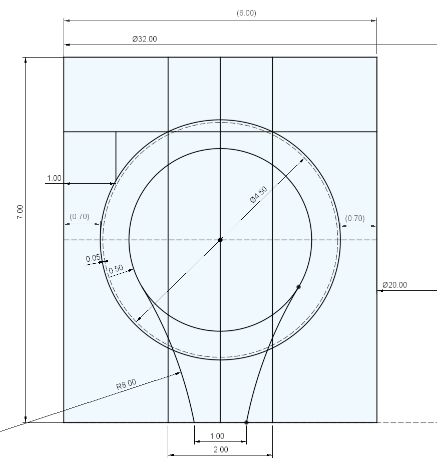
Every part except the ball pockets is a body of revolution, so the whole bearing is drawn in a single sketch on a plane through the axis and revolved four times, once per part. Drawing it this way puts all the running clearances in one place where they can be read against each other, rather than spreading them over four files. Figure 9.4.4 is that sketch.

Figure 9.4.4: The master cross-section. The axis of revolution lies to the right, so the right-hand edge is the \(\varnothing 20\) bore and the left-hand edge the \(\varnothing 32\) outside surface, and the reference dimension \((6.00)\) is the radial section. The dashed circle is the 4.5 mm ball, the arc \(0.05\) outside it is the race groove, and the arc a further \(0.50\) inside is the cage section. The two \((0.70)\) reference dimensions are the race walls, which fall out of those choices rather than being set. Along the bottom, \(2.00\) is the slot the cage skirt runs in and \(1.00\) the skirt itself.

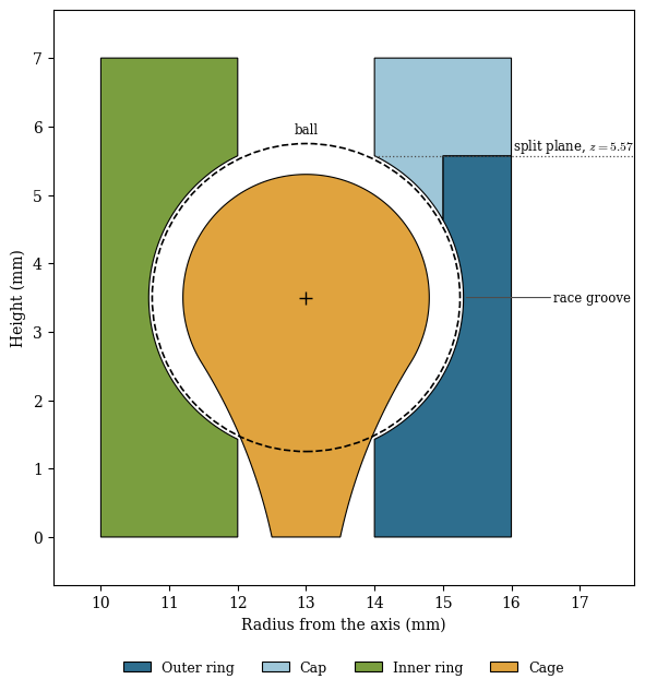
Four closed regions of that sketch are revolved separately, in the same way as the gear tooth is built by selecting contours rather than by trimming. Figure 9.4.5 redraws them from the dimensions above, which is also a check that the sketch closes.

Code
from scipy.optimize import brentq

z_m = B / 2                                        # ball centre height
r_si, r_so, r_cb = 12.0, 14.0, 15.0                # slot walls and cap counterbore
z_s = z_m + np.sqrt(r_g**2 - (r_so - r_m)**2)      # split plane of the outer race
z_l = z_m + np.sqrt(r_g**2 - (r_cb - r_m)**2)      # lower end of the cap lip
z_e = z_m - np.sqrt(r_g**2 - (r_so - r_m)**2)      # groove exit, lower side

def arc(r0, z0, R, a0, a1, n=240):
    # Points on an arc of radius R about (r0, z0), angles measured from the r axis
    a = np.linspace(a0, a1, n)
    return np.column_stack([r0 + R * np.cos(a), z0 + R * np.sin(a)])

def ang(r0, z0, r, z):
    return np.arctan2(z - z0, r - r0)

g = lambda r, z: ang(r_m, z_m, r, z)               # angle on the race groove

outer = np.vstack([[[D / 2, 0], [D / 2, z_s], [r_cb, z_s], [r_cb, z_l]],
                   arc(r_m, z_m, r_g, g(r_cb, z_l), g(r_so, z_e)),
                   [[r_so, 0]]])

cap = np.vstack([[[D / 2, B], [D / 2, z_s], [r_cb, z_s], [r_cb, z_l]],
                 arc(r_m, z_m, r_g, g(r_cb, z_l), g(r_so, z_s)),
                 [[r_so, B]]])

inner = np.vstack([[[d / 2, 0], [r_si, 0], [r_si, z_e]],
                   arc(r_m, z_m, r_g, g(r_si, z_e), g(r_si, z_s) - 2 * np.pi),
                   [[r_si, B], [d / 2, B]]])

# Cage: a circle 0.50 mm clear of the groove, flared to a 1.00 mm skirt by R8 arcs.
R_c, R_f, r_n = r_g - 0.50, 8.0, r_m + 0.5
centre = lambda th: (r_m + (R_c + R_f) * np.cos(th), z_m + (R_c + R_f) * np.sin(th))
th_t = brentq(lambda th: np.hypot(*np.subtract(centre(th), (r_n, 0.0))) - R_f, -1.2, -0.2)
a_f, b_f = centre(th_t)
P_t = (r_m + R_c * np.cos(th_t), z_m + R_c * np.sin(th_t))

flare = arc(a_f, b_f, R_f, ang(a_f, b_f, r_n, 0.0), ang(a_f, b_f, *P_t))
mirror = lambda p: np.column_stack([2 * r_m - p[:, 0], p[:, 1]])
cage = np.vstack([flare, arc(r_m, z_m, R_c, th_t, np.pi - th_t), mirror(flare[::-1])])

fig, ax = plt.subplots(figsize=(6.6, 6.4))
for poly, colour, name in [(outer, '#2E6E8E', 'Outer ring'), (cap, '#9EC6D8', 'Cap'),
                           (inner, '#7A9E3F', 'Inner ring'), (cage, '#E0A33E', 'Cage')]:
    ax.fill(poly[:, 0], poly[:, 1], color=colour, ec='k', lw=0.8, label=name, zorder=2)
ax.add_patch(plt.Circle((r_m, z_m), d_w / 2, fc='none', ec='k', ls='--', lw=1.2, zorder=4))
ax.plot(r_m, z_m, 'k+', ms=8, zorder=4)

ax.plot([r_so, 17.8], [z_s, z_s], color='0.3', ls=':', lw=0.9, zorder=5)
ax.annotate('split plane, $z = 5.57$', (17.8, z_s), xytext=(0, 4),
            textcoords='offset points', ha='right', fontsize=8.5)
ax.annotate('ball', (r_m, z_m + d_w / 2), xytext=(0, 7), textcoords='offset points',
            ha='center', fontsize=8.5, zorder=5)
ax.annotate('race groove', xy=(r_m + r_g, z_m), xytext=(17.75, z_m), ha='right',
            va='center', fontsize=8.5,
            arrowprops=dict(arrowstyle='-', lw=0.8, color='0.3',
                            shrinkA=0, shrinkB=2))

ax.set_aspect('equal')
ax.set_xlim(9.3, 17.8)
ax.set_ylim(-0.7, 7.7)
ax.set_xlabel('Radius from the axis (mm)')
ax.set_ylabel('Height (mm)')
ax.legend(fontsize=9, loc='upper center', bbox_to_anchor=(0.5, -0.11), ncol=4,
          frameon=False)
plt.tight_layout()
plt.show()
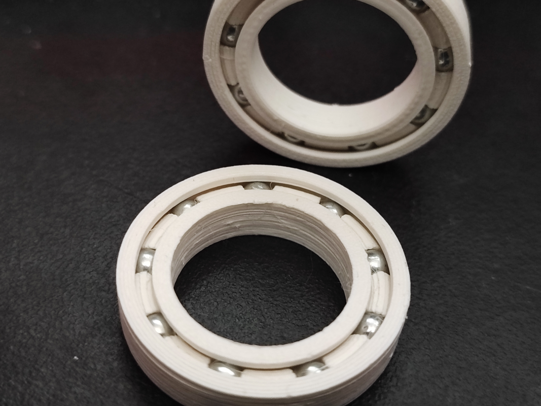
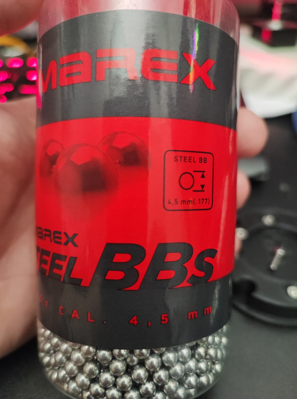
Figure 9.4.5: The four revolved profiles, rebuilt from the dimensions of Figure 9.4.4. The axis lies 9.4 mm to the left of the frame. The outer race is split at 5.57 mm, the height at which the groove arc reaches \(\varnothing 28\), and the cap carries the short lip above that plane. The cage section is a circle of radius 1.80 mm, everywhere 0.50 mm clear of the groove, flared to a 1.00 mm skirt that runs in the slot between the two rings.

The inner ring

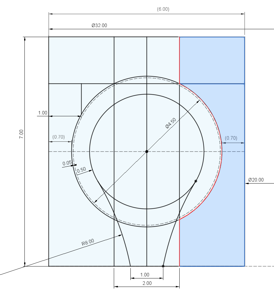
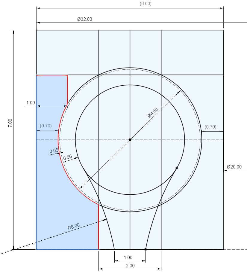
The inner ring is a sleeve from the \(\varnothing 20\) bore out to a land at \(\varnothing 24\), with the race groove cut into that land. The groove leaves the land 1.43 mm above the bottom face, reaches \(\varnothing 21.40\) at mid-width and returns to the land at 5.57 mm. Figure 9.4.6 shows the contour highlighted in the master sketch.

Figure 9.4.6: The inner ring contour. Its outside boundary is the land at \(\varnothing 24\) above and below, joined by the race groove. The \((0.70)\) reference dimension is the wall left between the bottom of the groove and the bore.

The outer ring

The outer ring mirrors it, running from \(\varnothing 32\) in to \(\varnothing 28\) with the groove reaching \(\varnothing 30.60\) at mid-width. Above the groove its bore opens out to a counterbore at \(\varnothing 30\), one millimetre below the outside surface, which is the seat the cap drops into. Figure 9.4.7 shows it.

Figure 9.4.7: The outer ring contour, ending at the split plane. The \(1.00\) dimension sets the counterbore one millimetre inside the outside surface, leaving an annular ledge for the cap to sit on and a wall thick enough to take the press fit.

The cap

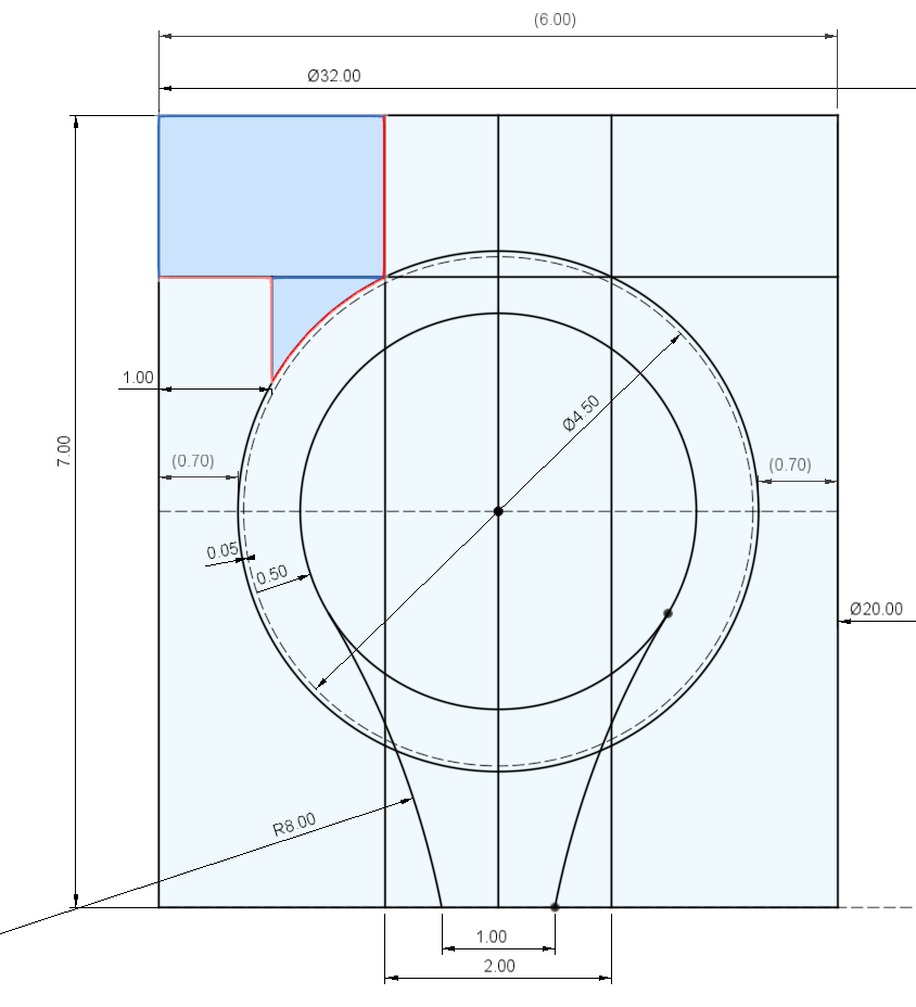
The outer race has to be split, because the groove is an undercut and nothing can be printed into it from above. The split is taken at 5.57 mm, the height where the groove arc crosses \(\varnothing 28\), and everything above that plane becomes a separate cap. The cap is stepped rather than flat: its outer part fills the \(\varnothing 30\) counterbore, which locates it radially, and a short lip reaches down past the split to carry the top of the groove. Figure 9.4.8 shows the profile.

Figure 9.4.8: The cap contour. The block above the split plane fills the counterbore out to \(\varnothing 32\), and the thin wedge below it is the lip that continues the race groove from \(\varnothing 30\) down to \(\varnothing 28\). Without that lip the ball would have nothing above it to run against.

The cage

The cage section is a circle of radius 1.80 mm about the ball centre, which keeps it 0.50 mm clear of the race groove the whole way round, carried down to the bottom face by two tangent arcs of radius 8 mm that close to a 1.00 mm skirt. Revolved, this is a ring with a skirt running in the 2.00 mm slot between the two race rings and clearing the slot walls by 0.05 mm where it is widest. Figure 9.4.9 highlights it.

A sphere centred on the ball centre is then cut from that ring and circular patterned nine times. The sphere is larger than the 3.60 mm section it cuts through, so each pocket opens on both sides and the ball is held by the web around its equator rather than enclosed. That is also what makes the cage flexible enough to assemble, as we come to below.

Figure 9.4.9: The cage contour. The upper circle sits inside the race groove with the \(0.50\) clearance dimensioned against it, and the \(R8.00\) arcs flare it down to the skirt at the bottom face. The skirt is what stops the cage from drifting sideways once the bearing is closed.

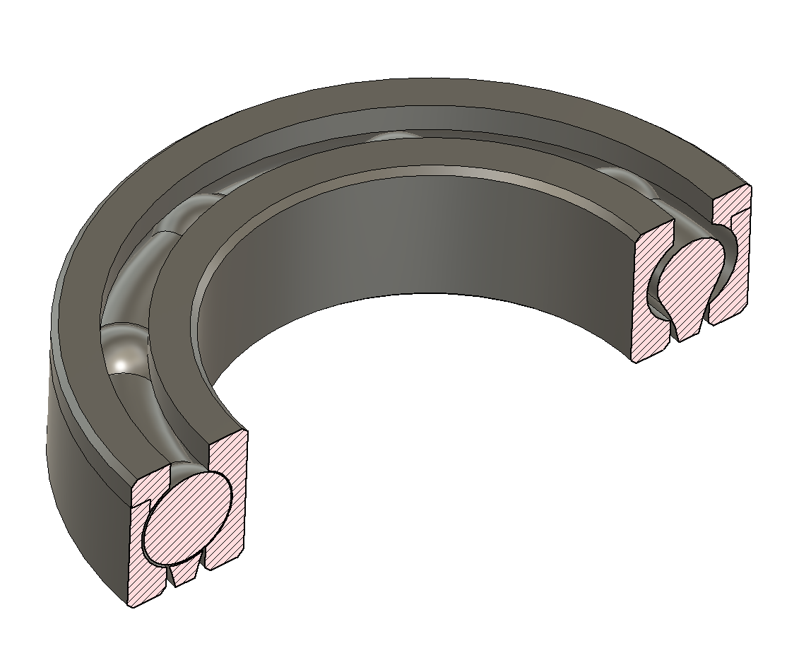
Revolving the four contours and cutting the pocket pattern gives Figure 9.4.10, which is the first point at which the design can be inspected rather than read.

Figure 9.4.10: Section view of the revolved assembly with one ball pocket cut. From the outside in: the outer ring, the cage with its skirt running in the slot, and the inner ring. The ball sits in the groove formed between the two rings, and the cap has been left off so the race is visible.

The two offsets that absorb the process

A printed hole comes out undersize and a printed boss oversize, because the extrudate shrinks as it cools and because the nozzle path is offset by half a line width in both cases. The error is worst on small diameters, where corner compensation and the widened first layer are a larger fraction of the feature. Rather than chase this through slicer settings, the model carries two offsets that are turned until the assembly runs.

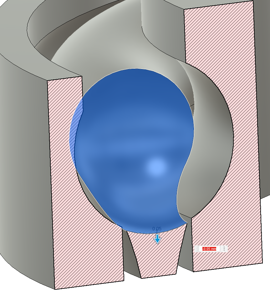
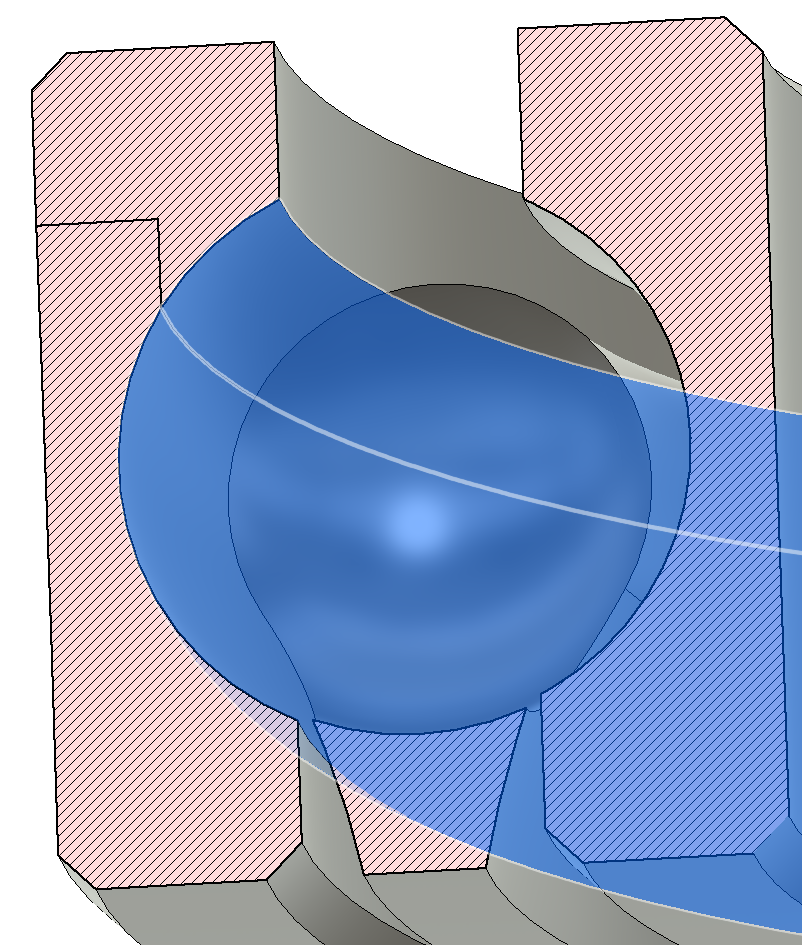
The first is on the spherical pocket in the cage. Shrinkage closes the pocket onto the ball and the cage seizes; offsetting the pocket face outwards opens it again. Figure 9.4.11 shows the field, set here to 0.05 mm.

The second is the bore of the outer ring above the race, the surface the rest of the assembly has to pass on its way in. A small bore pulls inwards as it cools, and offsetting that face outwards restores the fit, as in Figure 9.4.12.

Neither offset has a value that can be derived. They are set by printing the parts, assembling them, feeling the drag and changing the number, and the result holds for one printer with one material at one set of temperatures.

Figure 9.4.11: The pocket offset. The blue surface is the spherical cut that forms the ball pocket, and the handle applies a face offset of 0.05 mm to it. Too little and the cage grips the ball, too much and the ball rattles and the cage drifts off the pitch circle.
Figure 9.4.12: The bore offset. The large translucent surface is the bore of the outer ring above the race, highlighted with a ball shown in place for scale. This is the diameter the balls have to snap past during assembly, and it is the one most affected by shrinkage.

Assembly

The bearing goes together in one order only, and every step after the first is a snap fit whose interference follows from the geometry above.

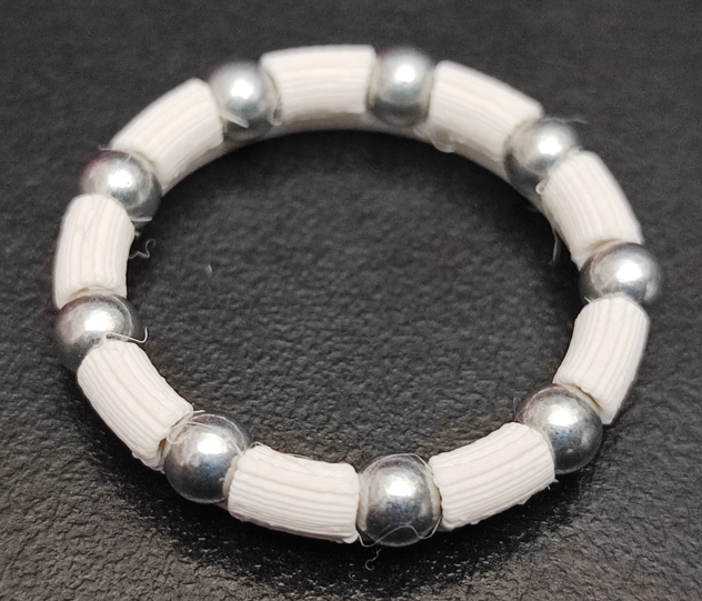
Start by pressing the nine balls into the cage from the open side of the pockets. They have to turn freely without falling out, which is what the pocket offset is for, and the result is Figure 9.4.13.

Figure 9.4.13: The cage with its nine balls fitted. Each ball stands proud on both faces because the pocket is larger than the cage section, and the webs between pockets hold them at the equator. The whiskers bridging the pockets are stringing from wet filament.

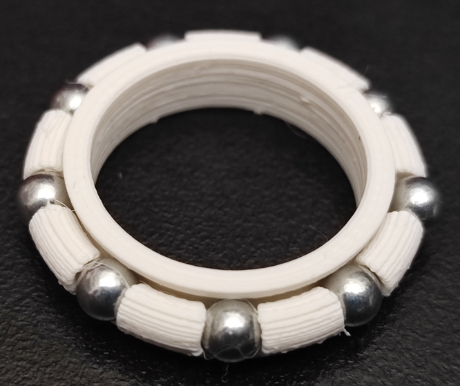
Next push the inner ring into the ring of balls. The balls reach \(\varnothing 21.50\) at their innermost point and the inner ring’s land measures \(\varnothing 24\), so this step drives 1.25 mm of radial interference past every ball at once. What gives is the cage: with nine spheres cut out of a 3.60 mm section it is a thin and very compliant ring, and it stretches far enough to let the land through before the balls drop into the groove. This is the step that decides whether a given print assembles at all, and it wants to be done slowly and squarely. Figure 9.4.14 is the result.

Figure 9.4.14: The inner ring pushed home. Its land is visible inside the ring of balls, and the balls have settled into the groove cut in it. Compare the ball spacing with Figure 9.4.13: the cage has returned to its free diameter.

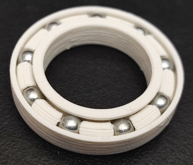
Then press that assembly into the outer ring. The throat here is the \(\varnothing 30\) counterbore against balls standing out to \(\varnothing 30.50\), so the interference is 0.25 mm on radius, a fifth of what the inner ring demanded, and the outer ring is the stiffer of the two parts. Figure 9.4.15 shows the bearing at this stage, complete except for the cap and with the race still open at the top.

Figure 9.4.15: The inner ring, cage and balls pressed into the outer ring. The balls sit in the groove and the top of the outer race is still open, which is why the bearing will come apart again if it is lifted by the inner ring.

Finally press the cap on, where it seats in the counterbore and closes the top of the race, giving Figure 9.4.16. Cyanoacrylate on the counterbore is optional and depends on where the bearing will be used: it is the only thing besides the press fit that holds the bearing together axially.

Run the bearing dry for a while first, then grease it. General purpose grease is fine.

Figure 9.4.16: The finished bearing with the cap pressed on. The joint line between cap and outer ring runs around the outside above the balls, and the bearing now behaves as one part.

Printing

Dry the filament before printing. The cage in Figure 9.4.13 was printed wet, and the whiskers bridging its pockets are the result. On a part whose running surfaces are a fraction of a millimetre across, a string in the wrong place is the difference between a bearing that turns and one that does not.

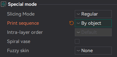
Print the four parts sequentially rather than side by side, one object finished before the next is started, using the print sequence setting in Figure 9.4.17. Printing them in parallel puts a travel move between parts on every layer, and every travel move is an opportunity to leave a blob on a race.

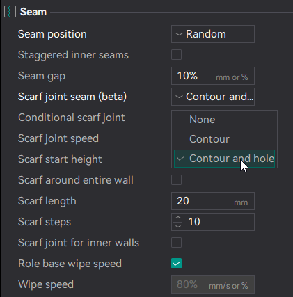
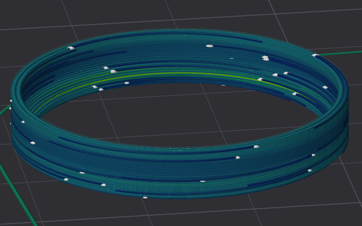
Set the seam to a random position and turn the scarf joint on, as in Figure 9.4.18. The seam is the small step left where a perimeter closes on itself, and on these parts almost every wall is a running surface. Randomising the position scatters those steps around the circumference instead of stacking them into a ridge up one side, and the scarf joint ramps the perimeter in and out over a length rather than stopping it abruptly. Figure 9.4.19 is the sliced result.

Figure 9.4.17: Print sequence set to by object. Each part is printed to full height before the next is started, which keeps the nozzle away from finished surfaces.
Figure 9.4.18: Seam settings: random seam position with the scarf joint applied to contours and holes. The scarf length and step count control how gradually the perimeter is ramped in and out.
Figure 9.4.19: The sliced outer ring. The pale marks scattered over the wall are the seam positions, spread around the circumference rather than aligned into a single ridge.

When to buy instead

Every dimension in this bearing came out of one inequality: the ball, two race walls and two running clearances have to fit inside the radial section. Turned round, that gives the largest ball a given envelope will take,

\[ d_w = \frac{D - d}{2} - 2t - 2c \tag{9.4.2}\]

with \(t\) the race wall and \(c\) the clearance. At \(t = 0.70\) mm and \(c = 0.05\) mm the 6804’s 6 mm section returns 4.5 mm, which is where the ball in this chapter came from.

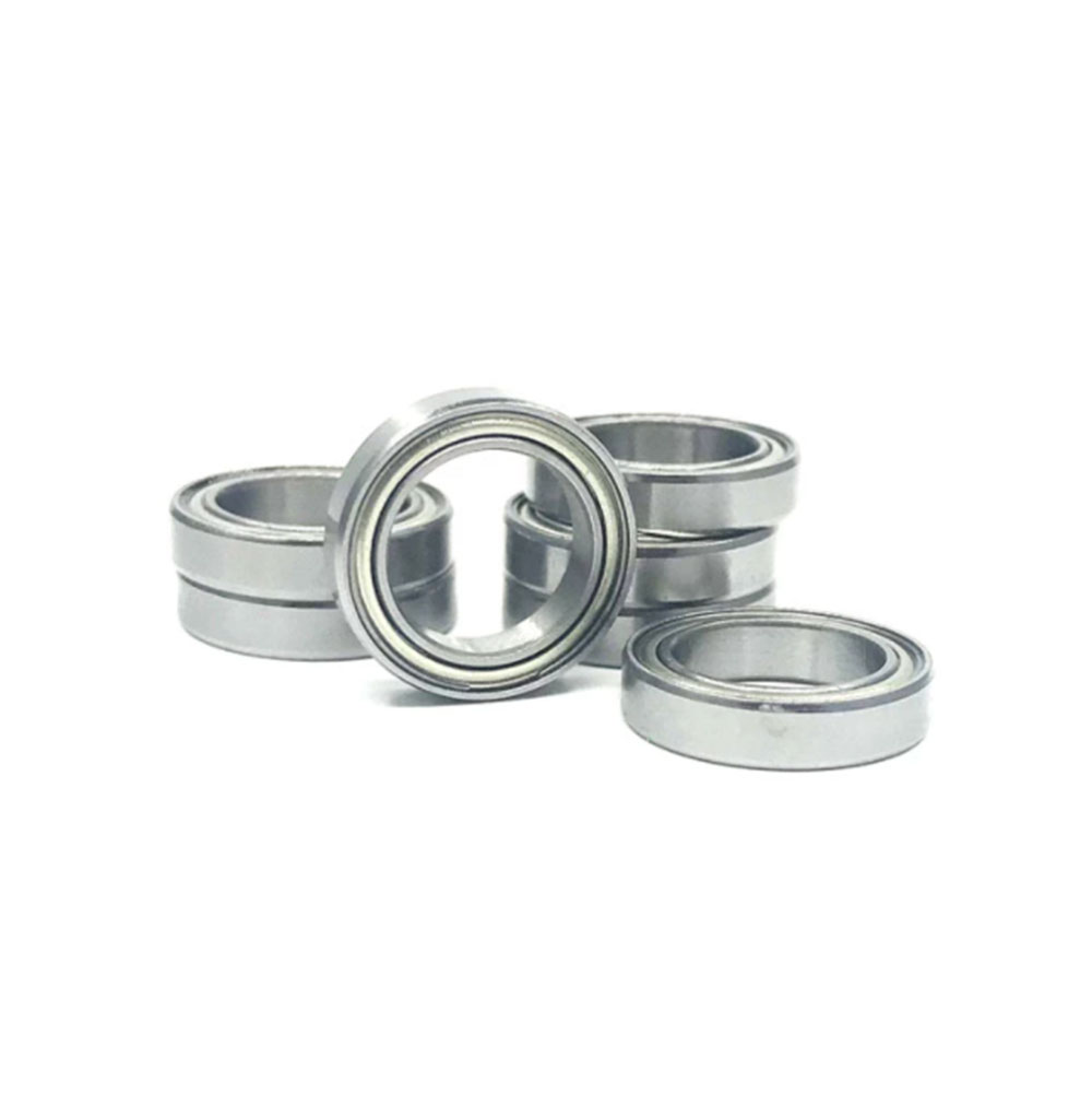
Neither \(t\) nor \(c\) is a property of the bearing. Both are set by the nozzle, and neither shrinks when the envelope does. On the 6804 they consume a quarter of the radial section. On the 12×18×4 bearings the course project buys by the packet, Figure 9.4.20, the section is 3 mm and they consume half of it, so 9.4.2 gives a ball of 1.5 mm.

Figure 9.4.20: Bought 12×18×4 shielded bearings, the size the course project stocks. Ground steel races, a hardened ball complement and a pressed steel shield on each face, for a price a printed bearing cannot approach once the failed attempts are counted. The one standing on edge shows the shield, which is what keeps the grease in and the swarf out.

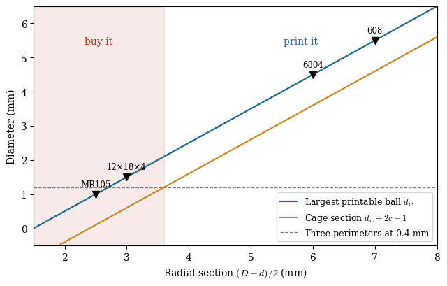
Ball spacing is not the constraint at that size: 9.4.1 allows 31 balls on the 7.5 mm pitch radius. What fails first is the cage. Subtracting the 0.50 mm race clearance from both sides of the ball leaves a cage section of \(d_w + 2c - 1.0\), and asking for three perimeters there puts the floor at a ball of 2.1 mm and a radial section of 3.6 mm. Figure 9.4.21 draws both limits against the envelopes worth comparing. The 12×18×4 sits below the floor: its cage would be 0.60 mm across, a single extruded line, with nine spherical pockets cut through it.

Code
t_wall = 0.70
section = np.linspace(1.5, 8.0, 200)
ball = section - 2 * t_wall - 2 * c
cage = ball + 2 * c - 1.0
sec_floor = w_cage + 2 * t_wall + 1.0    # section at which the cage reaches three perimeters

fig, ax = plt.subplots(figsize=(6.5, 4.2))
ax.plot(section, ball, color='#236B8E', lw=1.6, label='Largest printable ball $d_w$')
ax.plot(section, cage, color='#C98A2B', lw=1.6, label='Cage section $d_w + 2c - 1$')
ax.axhline(w_cage, color='0.5', ls='--', lw=0.9, label='Three perimeters at 0.4 mm')
ax.axvspan(1.5, sec_floor, color='#B5321E', alpha=0.10)
ax.annotate('buy it', ((1.5 + sec_floor) / 2, 5.4), ha='center', fontsize=10,
            color='#B5321E')
ax.annotate('print it', (5.8, 5.4), ha='center', fontsize=10, color='#236B8E')

for name, dd, DD in [('MR105', 5, 10), ('12×18×4', 12, 18), ('6804', 20, 32), ('608', 8, 22)]:
    sec = (DD - dd) / 2
    ax.plot(sec, sec - 2 * t_wall - 2 * c, 'v', ms=7, color='k')
    ax.annotate(name, (sec, sec - 2 * t_wall - 2 * c), xytext=(0, 8),
                textcoords='offset points', ha='center', fontsize=8.5)

ax.set_xlabel('Radial section $(D-d)/2$ (mm)')
ax.set_ylabel('Diameter (mm)')
ax.set_xlim(1.5, 8.0)
ax.set_ylim(-0.5, 6.5)
ax.legend(fontsize=9, loc='lower right')
plt.tight_layout()
plt.show()
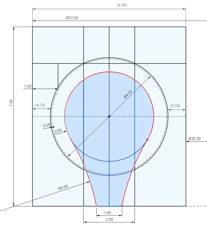
Figure 9.4.21: The printable ball and the cage section that follows from it, against the radial section of the envelope. The race wall and the running clearance are fixed by the printer, so both lines are straight and both hit zero at a finite section. Requiring three perimeters in the cage puts the crossover at a 3.6 mm section, which leaves the 6804 and the 608 comfortably printable and the 12×18×4 and the MR105 not. The 608 marker lands at 5.5 mm against the 5.556 mm ball a real 608 uses, which is a coincidence worth noticing and not a derivation.

There is a second reason to buy at that size, and it has nothing to do with geometry. The bought bearing arrives with ground races, a full hardened ball complement and a shield on each face, which is a specification the printed one does not attempt. What it also arrives with is a preservative grease heavy enough to dominate the running torque at the loads an RC car puts through a 12 mm bore, and whether flushing it for a light oil is worth doing is a measurement this course can make rather than a piece of received practice to repeat.

What the design still lacks

The bearing turns, carries a light radial load and costs almost nothing. What it does not have is a rating. The load a rolling bearing will take is governed by the contact between ball and race, and the standard treatment of that contact assumes both bodies are steel. Here one of them is a polymer with a modulus around one sixtieth of steel’s, a yield stress that falls off well below any temperature that troubles steel, and a layered structure whose strength depends on the direction the part was printed in. The catalogue formulas do not transfer, and the honest position is that we have a geometry that works and no number attached to it.

That is where the next version of this chapter has to go.

References

[1]
ISO 15:2017 Rolling bearings – Radial bearings – Boundary dimensions, general plan. Geneva, Switzerland: International Organization for Standardization; 2017.
[2]
Harris TA, Kotzalas MN. Rolling bearing analysis: Essential concepts of bearing technology. 5th ed. Boca Raton: CRC Press; 2006.