“The moment of the force of torsion is, for filaments of the same metal, proportional to the angle of twist, the fourth power of the diameter, and inversely proportional to the length of the filament.”
— Charles-Augustin de Coulomb, 1784, translated by A. K. T. Assis
Bending was the continuum model plus the assumption that cross sections stay plane and perpendicular to a bending axis. Torsion is the continuum model plus a different assumption: cross sections rotate rigidly about the axis of the shaft and stay plane while doing so. One assumption, one dimensional reduction, and the same three relations of Chapter 8.11 reappear with new names.
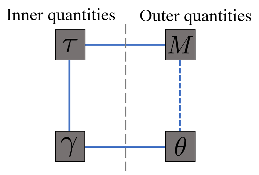
Figure 8.13.1: Rod quantities and shaft quantities in torsion, joined by the same three relations as in Figure 8.11.1.
The internal quantities are the shear stress \(\tau\) and the shear angle \(\gamma\), and the external ones are the applied torque \(M\) and the angle of twist \(\theta\). Everything below fills in the three arrows.
The kinematic assumption
Let \(x\) run along the shaft and let the cross section at \(x\) have rotated by an angle \(\theta(x)\) about that axis. A point at \((y, z)\) in the section is carried around with it, and for small angles a rotation by \(\theta\) moves it by \(\theta\) times its distance from the axis, perpendicular to the radius. The displacement field is therefore
\[
\bm u = \begin{bmatrix} 0 \\ -\theta(x)\, z \\ \theta(x)\, y \end{bmatrix}
\tag{8.13.1}\]
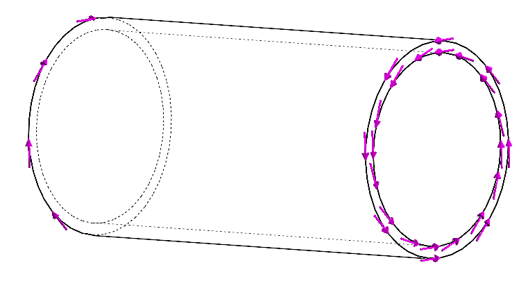
with no axial component, which is the statement that the section stays plane. Figure 8.13.2 shows what this looks like: longitudinal lines become helices while every circle stays a circle in its own plane.
Figure 8.13.2: A circular shaft under torsion. Cross sections rotate rigidly and remain plane.
⚠ Note
The assumption of no axial displacement is exact only for circular sections. Every other shape warps, meaning that points move out of the plane of the section, and the results below do not apply to it.
Strain and stress
The strain is the symmetric part of the displacement gradient, 8.7.3,
\[
\bm\varepsilon = \tfrac{1}{2}\left(\nabla\bm u + \nabla\bm u^\mathsf{T}\right)
\]
The rigid rotation of the section produces the antisymmetric entries \(-\theta\) and \(+\theta\) in the gradient, and those cancel in the symmetric part exactly as the rigid rotation did in Chapter 8.16. What survives is driven by the rate of twist\(d\theta/dx\),
with every other component zero. A shaft twisted uniformly along its length has a constant rate of twist; a shaft twisted at one end only would have \(d\theta/dx = 0\) and no strain anywhere, which is the correct statement that a rigid rotation of the whole shaft strains nothing.
Since the strain tensor has zero trace, the volumetric term in 8.9.7 drops out and the stress is pure shear,
\[
\bm\sigma = 2\mu\bm\varepsilon + \lambda\,\mathrm{tr}(\bm\varepsilon)\bm I = 2G\bm\varepsilon
\]
Code
sigma = sp.simplify(2*G*eps)ltx(r"\bm\sigma = 2\mu\bm\varepsilon +\lambda\,\mathrm{tr}(\bm\varepsilon)\bm I =", sigma)
\[ \bm\sigma = 2\mu\bm\varepsilon + \lambda\,\mathrm{tr}(\bm\varepsilon)\bm I =\left[\begin{matrix}0 & - G z \dfrac{d}{d x} \theta{\left(x \right)} & G y \dfrac{d}{d x} \theta{\left(x \right)}\\- G z \dfrac{d}{d x} \theta{\left(x \right)} & 0 & 0\\G y \dfrac{d}{d x} \theta{\left(x \right)} & 0 & 0\end{matrix}\right] \]
\[
\tau_{xy} = -G z \frac{d\theta}{dx}, \qquad \tau_{xz} = G y \frac{d\theta}{dx}
\]
The two components combine into a shear stress of magnitude \(G\rho\, d\theta/dx\) at radius \(\rho = \sqrt{y^2+z^2}\), directed tangentially. The stress therefore grows linearly from zero on the axis to a maximum at the surface,
The stress distribution must be statically equivalent to the applied torque. Each element of area \(dA\) at radius \(\rho\) carries a tangential force \(\tau\,dA\) acting with lever arm \(\rho\), so
\[
M = \int \rho\,\tau\, dA = \int \rho\,\frac{\rho}{R}\tau_{\max}\, dA
= \frac{\tau_{\max}}{R}\int \rho^2\, dA
\]
since \(\tau_{\max}/R\) is constant over the section. The remaining integral is a geometric property,
\[
\boxed{J = \int \rho^2\, dA}
\tag{8.13.4}\]
the polar second moment of area, the exact counterpart of \(I\) in 8.16.8 with the distance measured from the axis instead of from a neutral plane. Combining the two gives the stress at any radius and its maximum at the surface,
where \(W\) is the torsional section modulus, playing the same role for torsion that \(I/c\) played for bending. In polar coordinates \(dA = \rho\,d\rho\,d\varphi\), and 8.13.4 for a section between the radii \(R_i\) and \(R_o\) is
For a thin-walled tube of mean radius \(R\) and wall thickness \(t \ll R\) the integral collapses because every element sits at essentially the same radius, giving \(J = 2\pi R^3 t\) and \(W = 2\pi R^2 t\). That case is worth deriving separately, both as a check on the machinery and because it is the geometry in which torsion is used most efficiently.
A cross-check on the thin-walled tube
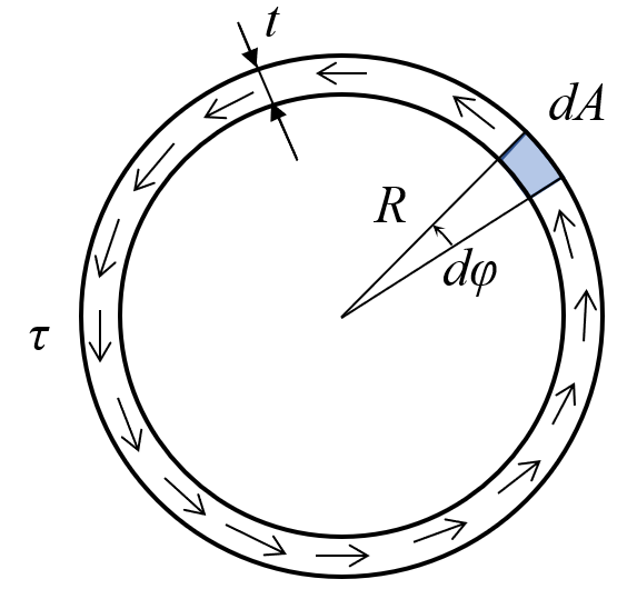
Figure 8.13.3 shows the section of a thin-walled shaft, with the shear stress running around the wall. Take a small strip subtending an angle \(d\varphi\).
Figure 8.13.3: A thin-walled shaft in torsion, and a strip of the wall subtending \(d\varphi\).
The strip has area \(dA = R\,d\varphi\, t\) when the wall is thin enough that we may roll it out flat, and it carries a tangential force \(T = \tau\, dA\) with lever arm \(R\), so its contribution to the torque is
which agrees with 8.13.5 and identifies \(W = 2\pi R^2 t\) as before.
Figure 8.13.4: A thin-walled shaft under torsion.
The angle of twist
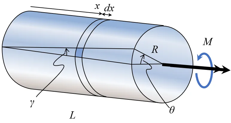
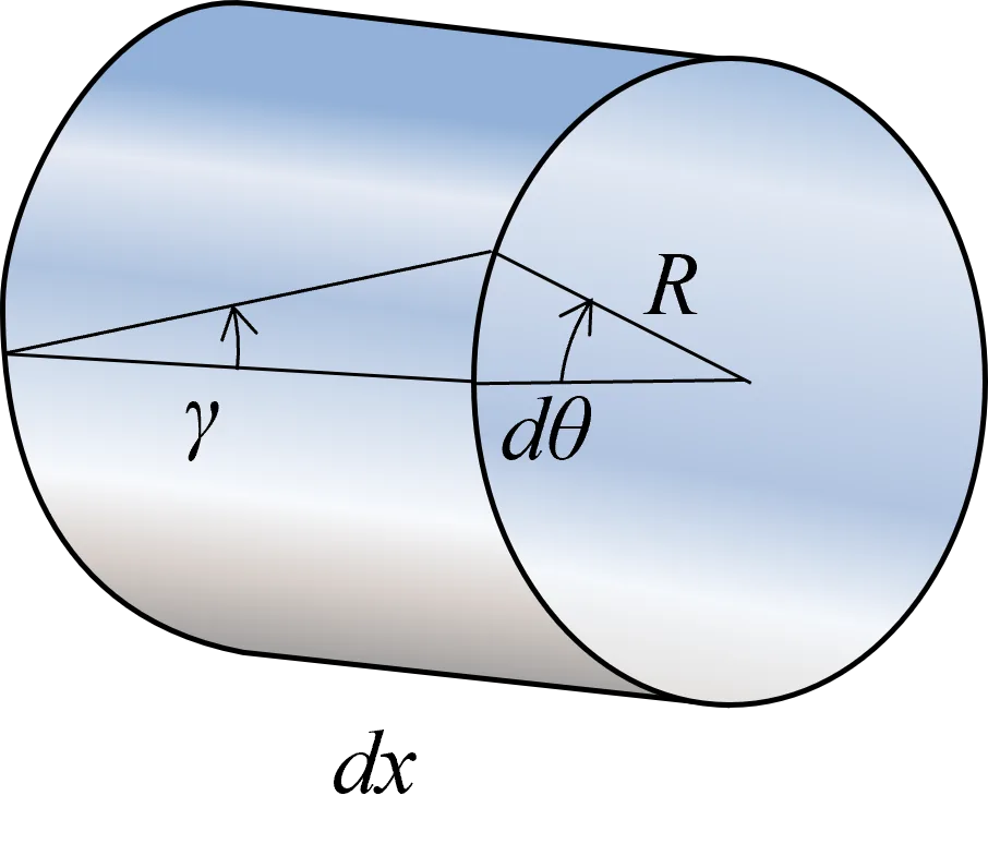
The last arrow of Figure 8.13.1 connects the shear angle to the angle of twist, and it is pure geometry. Figure 8.13.6 shows a slice of length \(dx\) whose far face has rotated by \(d\theta\) relative to the near one. A line on the surface that was parallel to the axis has tilted through the shear angle \(\gamma\), and the same arc length is described either way,
\[
\gamma\, dx = R\, d\theta
\tag{8.13.6}\]
Figure 8.13.5: The twisted shaft over its length \(L\)
Figure 8.13.6: A slice of length \(dx\)
Assuming linear elasticity, the material relation for shear is 8.5.11, \(\tau = G\gamma\), where the shear modulus is fixed by \(E\) and \(\nu\) through 8.9.5. Substituting into 8.13.6 and using 8.13.5 for the surface stress,
and integrating over the length of a uniform shaft gives
\[
\boxed{\theta = \frac{ML}{GJ}}
\tag{8.13.7}\]
The product \(GJ\) is the torsional rigidity, also called the torsional stiffness, the counterpart of the axial stiffness \(EA\) of 8.11.5 and the bending stiffness \(EI\) of 8.16.9. Where torque, material or section vary along the shaft, the integral must be kept,
which is the torsional analogue of the tapered rod of Chapter 8.12.
Example 1: Solid against hollow
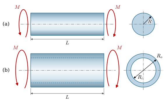
A steel shaft of length \(L = 1~\text{m}\) must transmit \(M = 500~\text{Nm}\). Compare a solid shaft of radius \(R = 20~\text{mm}\) with a hollow shaft of the same cross-sectional area, therefore the same mass per unit length, with outer radius \(R_o = 30~\text{mm}\), Figure 8.13.7. The shear modulus of steel is \(G = 81~\text{GPa}\). Which is stiffer, which is stronger, and by how much?
Figure 8.13.7: The two shafts of Example 1, each twisted by the torque \(M\) over the length \(L\). (a) Solid, of radius \(R\). (b) Hollow, of outer radius \(R_o\) and inner radius \(R_i\), with the same area as the solid section.
Equal area requires \(R_o^2 - R_i^2 = R^2\), which fixes the bore.
The hollow shaft is \(3.5\) times stiffer and carries \(2.3\) times less stress for the same mass of steel, because moving material outward increases \(\rho^2\) in 8.13.4 faster than it decreases the amount of material. This is the same argument that puts the flanges of an I-beam far from the neutral axis, and it is why drive shafts, bicycle frames and aircraft spars are tubes.
The other comparison keeps the same outer diameter. Boring the solid shaft out to an inner radius of half the outer removes \(25\,\%\) of the mass but only \((1/2)^4 = 6.25\,\%\) of \(J\), because the core sits near the axis where \(\rho^2\) is small and contributes little to the torsional rigidity. The surface stress rises by the same small amount, a factor of \(16/15\).
The gain is not free. A thin wall buckles under torsion long before it yields, so the wall thickness is eventually set by stability rather than by 8.13.5, and the tube must be joined to solid ends somehow. Both limits sit outside the model derived here.
Non-circular sections
Everything above rests on 8.13.1, and that field has no axial component. For a circular section this is exact, because the section has no way to distinguish one radial direction from another and therefore no reason to move out of plane. Any other section does warp, and a rectangular bar in torsion develops axial displacements that are largest at the corners.
The consequences are severe enough that the formulas must not be reused. The shear stress in a rectangular bar is zero at the corners, not maximum, and it peaks at the middle of the long side, which is the opposite of what 8.13.3 would predict. Handbooks tabulate approximate values of \(W\) and an effective \(J\) for common shapes, and the formulary carries a selection. Open thin-walled sections, a slit tube or a channel, are worse still: they are one to two orders of magnitude less stiff in torsion than the closed section of the same dimensions, because the shear flow has no closed path to run around.
Two thin-wall approximations put numbers on this. For thin-walled open sections, built from walls of width \(b\) and thickness \(t\), the effective polar moment is
linear in the width of each wall and cubic in its thickness. For a closed thin-walled section Bredt’s formula gives
\[
J = \frac{4A^2}{\oint ds/t}
\tag{8.13.10}\]
where \(A\) is the area enclosed by the midline of the wall and the integral runs once around that midline. A tube of radius \(R\) and wall \(t\) has \(J = 2\pi R^3 t\) closed and \(J \approx \tfrac{2}{3}\pi R t^3\) slit, a ratio of \(3(R/t)^2\), which is \(75\) for \(R/t = 5\).
Where accuracy matters for a non-circular section, the honest answer is to solve the continuum problem numerically. This is a case where the kinematic assumption that made the chapter possible is the very thing that fails, and where finite element analysis is not a convenience but the only correct route.