Body coordinates

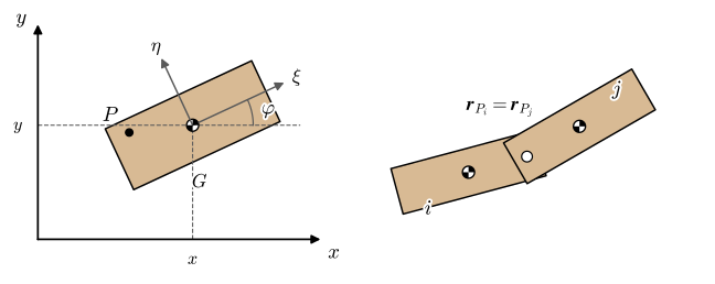
In the plane, a body is placed by the position \((x, y)\) of its centre of mass and its angle \(\varphi\) (Figure 7.10.1). For \(n\) bodies the three coordinates of each are collected in one vector,

\[ \bm q = \begin{bmatrix} x_1 & y_1 & \varphi_1 & \cdots & x_n & y_n & \varphi_n \end{bmatrix}^\mathsf{T} , \]

with \(3n\) entries. These body coordinates can describe any arrangement of the bodies, including a mechanism taken apart. A point \(P\) fixed in body \(i\) has constant local coordinates \(\bm s'_P = [\xi_P,\ \eta_P]^\mathsf{T}\) in the body’s frame, and its global position is the centre of mass plus the local vector turned by the body’s angle,

\[ \bm r_P = \begin{bmatrix} x_i \\ y_i \end{bmatrix} + \bm A(\varphi_i)\,\bm s'_P , \qquad \bm A(\varphi) = \begin{bmatrix} \cos\varphi & -\sin\varphi \\ \sin\varphi & \cos\varphi \end{bmatrix} . \tag{7.10.1}\]

Joints as constraint equations

Every joint is written as one or more equations that are zero when the joint is assembled, collected in the constraint vector \(\bm C(\bm q, t) = \bm 0\). A pin joint between the points \(P_i\) of body \(i\) and \(P_j\) of body \(j\) requires the two points to coincide (Figure 7.10.1), two scalar equations from 7.10.1,

\[ \bm r_{P_i}(x_i, y_i, \varphi_i) - \bm r_{P_j}(x_j, y_j, \varphi_j) = \bm 0 , \]

and a pin to the ground replaces \(\bm r_{P_j}\) by a fixed point. A body that slides along the \(x\)-axis without turning, a translational joint to the ground, has \(y_i = 0\) and \(\varphi_i = 0\). A motor that turns body \(i\) by a prescribed angle adds a driving constraint, \(\varphi_i - f(t) = 0\), which depends on time. A mechanism with \(3n\) coordinates and \(m\) independent constraints has \(3n - m\) degrees of freedom.

Kinematic analysis

When the driving constraints use up the degrees of freedom, there are as many equations as coordinates, and the position of the mechanism at the time \(t\) is the root of \(\bm C(\bm q, t) = \bm 0\). The equations are nonlinear, and the Newton-Raphson method solves them by repeated linearisation around a guess \(\bm q_k\),

\[ \bm J(\bm q_k)\,\Delta\bm q = -\bm C(\bm q_k, t) , \qquad \bm q_{k+1} = \bm q_k + \Delta\bm q , \qquad \bm J = \frac{\partial\bm C}{\partial\bm q} , \tag{7.10.2}\]

where the constraint Jacobian \(\bm J\) holds the derivative of every constraint with respect to every coordinate. The velocities and accelerations follow from differentiating \(\bm C(\bm q(t), t) = \bm 0\) in time, once and twice:

\[ \bm J\dot{\bm q} = -\bm C_t , \qquad \bm J\ddot{\bm q} = \bm\gamma , \qquad \bm\gamma = -\bigl(\bm J\dot{\bm q}\bigr)_{\bm q}\,\dot{\bm q} - 2\bm C_{t\bm q}\,\dot{\bm q} - \bm C_{tt} , \tag{7.10.3}\]

where subscripts denote partial derivatives. Both are linear systems with the same matrix \(\bm J\). The vector \(\bm\gamma\) holds the centripetal and Coriolis terms of the joints, and for constraints without time it reduces to \(-\dot{\bm J}\dot{\bm q}\).

The solver below builds \(\bm C\) from a list of joints, lets SymPy differentiate it into \(\bm J\), \(\bm C_t\) and \(\bm\gamma\), and turns them into numerical functions. A commercial program does the same with hand-coded derivatives for each joint type.

t = sp.symbols('t', real=True)

class Mechanism:
    """A planar multibody model in body coordinates (x, y, phi) of each centre of mass."""

    def __init__(self):
        self.bodies, self.cons = [], []

    def body(self, name, m, I):
        q = sp.symbols(f'x_{name} y_{name} phi_{name}', real=True)
        self.bodies.append(dict(m=m, I=I, q=q))
        return len(self.bodies) - 1

    def point(self, b, s):                       # eq-ms-point
        x, y, ph = self.bodies[b]['q']
        A = sp.Matrix([[sp.cos(ph), -sp.sin(ph)], [sp.sin(ph), sp.cos(ph)]])
        return sp.Matrix([x, y]) + A*sp.Matrix(s)

    def pin(self, b1, s1, b2=None, s2=None, ground=(0, 0)):
        p2 = self.point(b2, s2) if b2 is not None else sp.Matrix(ground)
        self.cons += list(self.point(b1, s1) - p2)

    def add(self, expr):                         # any other constraint, e.g. a driver
        self.cons.append(expr)

    def build(self):
        q = sp.Matrix([c for b in self.bodies for c in b['q']])
        qd = sp.Matrix(sp.symbols(f'qd0:{len(q)}', real=True))
        C = sp.Matrix(self.cons)
        J = C.jacobian(q)
        Ct = C.diff(t)
        gamma = -(J*qd).jacobian(q)*qd - 2*Ct.jacobian(q)*qd - Ct.diff(t)     # eq-ms-vel-acc
        f = lambda e: sp.lambdify((q, qd, t), e, 'numpy')
        self.C_f, self.J_f, self.Ct_f, self.g_f = f(C), f(J), f(Ct), f(gamma)
        self.M = np.diag([v for b in self.bodies for v in (b['m'], b['m'], b['I'])])
        self.n, self.m = len(q), len(C)
        return self

    def C(self, q, qd, t_):  return np.asarray(self.C_f(q, qd, t_), float).ravel()
    def J(self, q, qd, t_):  return np.asarray(self.J_f(q, qd, t_), float)
    def Ct(self, q, qd, t_): return np.asarray(self.Ct_f(q, qd, t_), float).ravel()
    def gamma(self, q, qd, t_): return np.asarray(self.g_f(q, qd, t_), float).ravel()

    def kinematics(self, q, t_):
        """Position by Newton-Raphson, then velocity and acceleration (driven mechanism)."""
        z = np.zeros(self.n)
        for _ in range(30):
            dq = np.linalg.solve(self.J(q, z, t_), -self.C(q, z, t_))
            q = q + dq
            if np.linalg.norm(dq) < 1e-13:
                break
        J = self.J(q, z, t_)
        qd = np.linalg.solve(J, -self.Ct(q, z, t_))
        return q, qd, np.linalg.solve(J, self.gamma(q, qd, t_))

    def accel(self, q, qd, t_, f_ext):
        """Solve the block system for the accelerations and the multipliers (eq-ms-dae)."""
        J = self.J(q, qd, t_)
        A = np.block([[self.M, J.T], [J, np.zeros((self.m, self.m))]])
        sol = np.linalg.solve(A, np.concatenate([f_ext(q, qd, t_), self.gamma(q, qd, t_)]))
        return sol[:self.n], sol[self.n:]

    def project(self, q, qd, t_):
        """Pull the state back onto the constraints: positions, then velocities (eq-ms-project)."""
        for _ in range(20):
            Cv = self.C(q, qd, t_)
            if np.linalg.norm(Cv) < 1e-12:
                break
            J = self.J(q, qd, t_)
            q = q - J.T @ np.linalg.solve(J @ J.T, Cv)
        J, Minv = self.J(q, qd, t_), np.diag(1/np.diag(self.M))
        mu = np.linalg.solve(J @ Minv @ J.T, -(J @ qd + self.Ct(q, qd, t_)))
        return q, qd + Minv @ J.T @ mu

    def simulate(self, q0, qd0, f_ext, T, dt, project=True):
        """Euler-Cromer in time, with or without the projection step."""
        n = int(T/dt)
        Q, QD, LAM = np.zeros((n, self.n)), np.zeros((n, self.n)), np.zeros((n, self.m))
        q, qd = np.array(q0, float), np.array(qd0, float)
        for i in range(n):
            qdd, lam = self.accel(q, qd, i*dt, f_ext)
            Q[i], QD[i], LAM[i] = q, qd, lam
            qd = qd + dt*qdd
            q = q + dt*qd
            if project:
                q, qd = self.project(q, qd, (i + 1)*dt)
        return np.arange(n)*dt, Q, QD, LAM

Example 1: The crank-slider, kinematics

The crank-slider of Example 11 in Particle kinematics has the crank \(OB\) of length \(r = 125\) mm, turning at \(\omega = 25\) rad/s, the rod \(AB\) of length \(L = 350\) mm with its centre of mass 100 mm from \(B\), and the slider \(A\) on the line through \(O\) (Figure 7.8.1). The kinematics chapter found the slider position \(x_A(\theta)\) in closed form; here the solver finds it from the joints alone.

The model has three bodies and nine coordinates. The crank (body 1) has its centre halfway along it, so its pin to the ground is at \(\bm s' = [-r/2,\ 0]^\mathsf{T}\) and its pin to the rod at \([r/2,\ 0]^\mathsf{T}\). The rod (body 2) has its local \(\xi\)-axis from \(B\) towards \(A\), so \(B\) is at \([-0.1,\ 0]^\mathsf{T}\) m and \(A\) at \([0.25,\ 0]^\mathsf{T}\) m. The slider (body 3) is pinned to the rod at its centre and slides on the \(x\)-axis. The crank angle of the kinematics chapter, \(\theta\) from the negative \(x\)-axis upwards, is \(\theta = \pi - \varphi_1\), so the motor drives \(\varphi_1 = \pi - \omega t\). That gives nine constraints:

\[ \underbrace{\bm r_{O,1} = \bm 0}_{2} , \quad \underbrace{\bm r_{B,1} = \bm r_{B,2}}_{2} , \quad \underbrace{\bm r_{A,2} = \bm r_{A,3}}_{2} , \quad \underbrace{y_3 = 0 ,\ \varphi_3 = 0}_{2} , \quad \underbrace{\varphi_1 - (\pi - \omega t) = 0}_{1} . \]

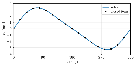
We solve 7.10.2 and 7.10.3 at 73 instants of one revolution and compare the slider with the closed form, \(x_A = -\bigl(r\cos\theta + \sqrt{L^2 - r^2\sin^2\theta}\bigr)\) and \(\dot x_A = \omega\,dx_A/d\theta\).

r_c, L_r, BG, om = 0.125, 0.35, 0.10, 25.0

def crank_slider(m_c=1e-6, m_r=1e-6, m_s=1e-6, omega=om):
    mech = Mechanism()
    c = mech.body('c', m_c, m_c*r_c**2/12)
    rod = mech.body('r', m_r, m_r*L_r**2/12)
    s = mech.body('s', m_s, m_s*1e-3)
    mech.pin(c, (-r_c/2, 0))                              # crank to ground at O
    mech.pin(c, (r_c/2, 0), rod, (-BG, 0))                # crank to rod at B
    mech.pin(rod, (L_r - BG, 0), s, (0, 0))               # rod to slider at A
    mech.add(mech.bodies[s]['q'][1])                      # slider on the x-axis
    mech.add(mech.bodies[s]['q'][2])                      # without turning
    mech.add(mech.bodies[c]['q'][2] - (sp.pi - omega*t))  # the motor
    return mech.build()

q_start = np.array([-r_c/2, 0, np.pi, -r_c - BG, 0, np.pi, -(r_c + L_r), 0, 0.0])
cs = crank_slider()
q = q_start.copy()
rows = []
for t_ in np.linspace(0, 2*np.pi/om, 73):
    q, qd, qdd = cs.kinematics(q, t_)
    th = om*t_
    root = np.sqrt(L_r**2 - (r_c*np.sin(th))**2)
    rows.append((th, q[6], qd[6], -(r_c*np.cos(th) + root), om*r_c*np.sin(th)*(1 + r_c*np.cos(th)/root)))
rows = np.array(rows)
err_x, err_v = np.max(np.abs(rows[:, 1] - rows[:, 3])), np.max(np.abs(rows[:, 2] - rows[:, 4]))

The largest differences between the solver and the closed form over the revolution are

fig, ax = plt.subplots(figsize=(6, 3))
ax.plot(np.degrees(rows[:, 0]), rows[:, 2], color='C0', lw=2, label='solver')
ax.plot(np.degrees(rows[::4, 0]), rows[::4, 4], 'ko', ms=4, label='closed form')
ax.set_xlabel(r'$\theta$ [deg]'); ax.set_ylabel(r'$\dot x_A$ [m/s]'); ax.grid(alpha=0.3)
ax.set_xlim(0, 360); ax.set_xticks([0, 90, 180, 270, 360]); ax.set_ylim(-4, 4)
ax.legend(loc='upper right', fontsize=9)
end_ticks(fig)
plt.tight_layout(); plt.show()

The solver reproduces the closed form to rounding error. It never used the geometry of the triangle \(OBA\) that the kinematics chapter solved by hand: three pins, a guide and a motor were enough.

The equations of motion

Each free body obeys Newton’s and Euler’s laws, which for all bodies together read \(\bm M\ddot{\bm q} = \bm f + \bm f_c\). The mass matrix \(\bm M\) is diagonal, with \(m_i\), \(m_i\) and \(\bar I_i\) for the three coordinates of body \(i\). The vector \(\bm f\) holds the applied forces: gravity, springs, dampers and loads, each reduced to a force at the centre of mass and a moment, as below. The vector \(\bm f_c\) holds the unknown forces of the joints.

The joints are ideal, so by Virtual work their forces do no work in any virtual displacement the joints allow: \(\bm f_c^\mathsf{T}\delta\bm q = 0\) for every \(\delta\bm q\) with \(\bm J\,\delta\bm q = \bm 0\). A vector that is orthogonal to every solution of \(\bm J\,\delta\bm q = \bm 0\) is a combination of the rows of \(\bm J\), so

\[ \bm f_c = -\bm J^\mathsf{T}\bm\lambda , \]

with one Lagrange multiplier \(\lambda_k\) for each constraint equation, the size of the force that enforces it. The minus sign is a convention. Adding the acceleration condition of 7.10.3 gives as many equations as unknowns, the accelerations and the multipliers together:

\[ \begin{bmatrix} \bm M & \bm J^\mathsf{T} \\ \bm J & \bm 0 \end{bmatrix} \begin{bmatrix} \ddot{\bm q} \\ \bm\lambda \end{bmatrix} = \begin{bmatrix} \bm f \\ \bm\gamma \end{bmatrix} . \tag{7.10.4}\]

This is the core of the solver. At any instant, with the positions and velocities known, it is one linear system; its solution gives the accelerations of every body and the force in every joint. For a pin joint the two multipliers are, with the opposite sign, the components of the pin force on the first body. For a driving constraint the multiplier is the moment of the motor. The differential equations of motion and the algebraic constraint equations together form a system of differential-algebraic equations.

Applied forces

A force \(\bm F\) at the point \(P\) of body \(i\) enters \(\bm f\) as the force \(\bm F\) on \((x_i, y_i)\) and the moment of \(\bm F\) about the centre of mass on \(\varphi_i\),

\[ \bm f_i = \begin{bmatrix} F_x \\ F_y \\ (\bm A\bm s'_P)_x F_y - (\bm A\bm s'_P)_y F_x \end{bmatrix} . \]

A spring and damper between a point on body \(i\) and a point on body \(j\), with the current length \(\ell\) and the rate \(\dot\ell\), pulls with \(F = k(\ell - \ell_0) + c\dot\ell\) along the line between the points, which enters as two such forces, equal and opposite. Gravity acts at the centres of mass and contributes only \(-m_ig\) to the \(y_i\) entries.

Example 2: The moment of the motor

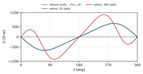
The crank-slider of Example 1 now carries the piston force \(P = 5\) kN on the slider, towards \(O\), as in Example 1 in Virtual work, and the motor holds the crank at \(\omega = 25\) rad/s. The mechanism has no degree of freedom left, so its motion is known from the kinematics, and 7.10.4 with the known accelerations gives the multipliers: the problem of inverse dynamics. The multiplier of the driving constraint \(\varphi_1 - (\pi - \omega t)\) is the motor moment in the sense of increasing \(\theta\), the moment \(M\) of the virtual work chapter.

With parts of negligible mass the moment must be the virtual work result, \(M = -P\,dx_A/d\theta\). With real parts, a crank of 1.0 kg, a rod of 0.8 kg and a slider of 0.5 kg, the inertia of the moving parts adds to it, and the more so the faster the crank turns. We compare 25 rad/s with 300 rad/s, about 2900 rpm.

P_gas = 5000.0
f_piston = lambda q, qd, t_: np.array([0, 0, 0, 0, 0, 0, P_gas, 0, 0.0])

def motor_moment(mech, omega, n_pts=181):
    q, out = q_start.copy(), []
    for t_ in np.linspace(0, 2*np.pi/omega, n_pts):
        q, qd, _ = mech.kinematics(q, t_)
        _, lam = mech.accel(q, qd, t_, f_piston)
        out.append((omega*t_, lam[-1]))
    return np.array(out)

light = motor_moment(crank_slider(), om)
th_m = light[:, 0]
M_vw = -P_gas*r_c*np.sin(th_m)*(1 + r_c*np.cos(th_m)/np.sqrt(L_r**2 - (r_c*np.sin(th_m))**2))
real = {w: motor_moment(crank_slider(1.0, 0.8, 0.5, w), w) for w in (25.0, 300.0)}
diff_light = np.max(np.abs(light[:, 1] - M_vw))
add_inertia = {w: np.max(np.abs(real[w][:, 1] - M_vw)) for w in real}

The multiplier of the motor, against the moment from virtual work, and the largest contribution of the inertia at the two speeds:

fig, ax = plt.subplots(figsize=(6, 3.2))
ax.plot(np.degrees(th_m), M_vw, 'k', lw=3, alpha=0.3, label=r'virtual work, $-P\,dx_A/d\theta$')
ax.plot(np.degrees(real[25.0][:, 0]), real[25.0][:, 1], color='C0', lw=1.5, label='solver, 25 rad/s')
ax.plot(np.degrees(real[300.0][:, 0]), real[300.0][:, 1], color='C3', lw=1.5, label='solver, 300 rad/s')
ax.axhline(0, color='k', lw=0.6)
ax.set_xlabel(r'$\theta$ [deg]'); ax.set_ylabel(r'$M$ [N$\cdot$m]'); ax.grid(alpha=0.3)
ax.set_xlim(0, 360); ax.set_xticks([0, 90, 180, 270, 360]); ax.set_ylim(-1200, 1200)
ax.legend(loc='lower center', bbox_to_anchor=(0.5, 1.0), ncol=2, fontsize=8, frameon=False)
end_ticks(fig)
plt.tight_layout(); plt.show()

With light parts the multiplier is the virtual work moment to rounding error: the moment a motor must deliver is a Lagrange multiplier. At 25 rad/s the inertia of the real parts changes the moment by a few newton metres out of 664. At 300 rad/s it adds almost 800 N·m, and the moment changes sign twice more per revolution, near \(55^\circ\) and \(305^\circ\): there the slider and the rod, braking, drive the crank, and the motor has to hold them back. The moment still vanishes at the dead centres, where the slider stands still and its inertia force has no lever on the crank. This is why the virtual work result, which ignores the masses, serves for slow mechanisms and why engines need the full dynamics.

Time integration and drift

A mechanism with degrees of freedom left moves under its forces, and 7.10.4 is integrated in time. With the Euler-Cromer method of the earlier chapters, each step solves 7.10.4 for \(\ddot{\bm q}\) and then updates

\[ \dot{\bm q}_{i+1} = \dot{\bm q}_i + \Delta t\,\ddot{\bm q}_i , \qquad \bm q_{i+1} = \bm q_i + \Delta t\,\dot{\bm q}_{i+1} . \]

The solver enforces the joints only through the acceleration condition \(\bm J\ddot{\bm q} = \bm\gamma\), twice differentiated. The integration errors in the velocities and positions are not corrected by it, so the joints slowly come apart: the positions drift off \(\bm C = \bm 0\) and the velocities off \(\bm J\dot{\bm q} = -\bm C_t\). A practical solver therefore projects the state back after each step. The positions are corrected by Newton iterations of the smallest size that satisfy the constraints, and the velocities by the smallest correction, measured with the mass matrix, that satisfies their constraint:

\[ \bm q \leftarrow \bm q - \bm J^\mathsf{T}\bigl(\bm J\bm J^\mathsf{T}\bigr)^{-1}\bm C , \qquad \dot{\bm q} \leftarrow \dot{\bm q} + \bm M^{-1}\bm J^\mathsf{T}\bm\mu , \quad \bigl(\bm J\bm M^{-1}\bm J^\mathsf{T}\bigr)\bm\mu = -\bigl(\bm J\dot{\bm q} + \bm C_t\bigr) , \tag{7.10.5}\]

the position correction repeated until \(\bm C\) vanishes. Projection keeps the joints closed. It does not remove the error of the time integration itself, which the energy check measures as before.

Example 3: The bar pendulum, and why projection is needed

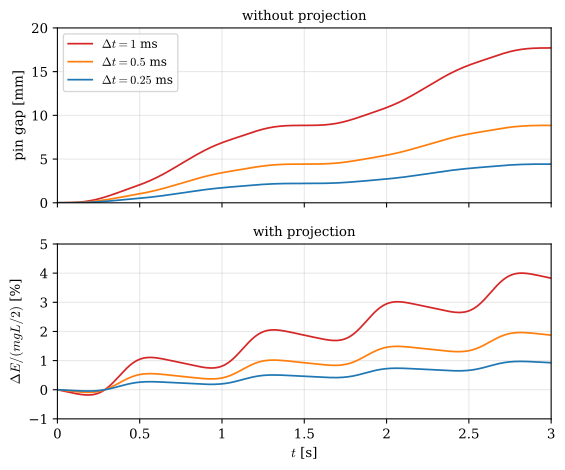
The bar pendulum of Example 1 in Rigid body kinetics, \(L = 0.6\) m and \(m = 1.2\) kg, without pin friction, is one body with a pin to the ground at its end, \(\bm s' = [-L/2,\ 0]^\mathsf{T}\): three coordinates, two constraints, one degree of freedom (Figure 7.6.2). It starts horizontal, \(\varphi = 0\), at rest, and we integrate three seconds with three time steps, first without the projection of 7.10.5 and then with it. Without projection we measure how far the end of the bar has moved away from the pin; with it, the drift of the energy \(E = \tfrac12 m(\dot x^2 + \dot y^2) + \tfrac12\bar I\dot\varphi^2 + mgy\), as in Work, energy and power.

g = 9.81
L_b, m_b = 0.6, 1.2
pend = Mechanism()
bar = pend.body('b', m_b, m_b*L_b**2/12)
pend.pin(bar, (-L_b/2, 0))
pend.build()
f_grav = lambda q, qd, t_: np.array([0, -m_b*g, 0.0])

def bar_energy(Q, QD):
    return m_b*(QD[:, 0]**2 + QD[:, 1]**2)/2 + m_b*L_b**2/24*QD[:, 2]**2 + m_b*g*Q[:, 1]

study = {}
for dt_ in (1e-3, 5e-4, 2.5e-4):
    _, Qf, QDf, _ = pend.simulate([L_b/2, 0, 0], [0, 0, 0], f_grav, T=3.0, dt=dt_, project=False)
    gap = np.hypot(Qf[:, 0] - L_b/2*np.cos(Qf[:, 2]), Qf[:, 1] - L_b/2*np.sin(Qf[:, 2]))
    tp, Qp, QDp, LAMp = pend.simulate([L_b/2, 0, 0], [0, 0, 0], f_grav, T=3.0, dt=dt_)
    Ep = bar_energy(Qp, QDp)
    study[dt_] = dict(t=tp, gap=gap, drift=(Ep - Ep[0])/(m_b*g*L_b/2), Q=Qp, LAM=LAMp)

fig, axes = plt.subplots(2, 1, figsize=(6, 5), sharex=True)
for (dt_, s_), col in zip(study.items(), ('C3', 'C1', 'C0')):
    axes[0].plot(s_['t'], 1e3*s_['gap'], color=col, lw=1.3, label=rf'$\Delta t = {1e3*dt_:g}$ ms')
    axes[1].plot(s_['t'], 100*s_['drift'], color=col, lw=1.3)
axes[0].set_ylabel('pin gap [mm]'); axes[0].set_ylim(0, 20); axes[0].legend(loc='upper left', fontsize=9)
axes[0].set_title('without projection', fontsize=10)
axes[1].set_ylabel(r'$\Delta E/(mgL/2)$ [%]'); axes[1].set_ylim(-1, 5); axes[1].set_xlabel('$t$ [s]')
axes[1].set_title('with projection', fontsize=10)
for a in axes: a.grid(alpha=0.3); a.set_xlim(0, 3)
end_ticks(fig)
plt.tight_layout(); plt.show()

fine = study[2.5e-4]
theta_fine = fine['Q'][:, 2] + np.pi/2
i_bot = np.argmin(np.abs(theta_fine[fine['t'] < 0.6]))
R_bottom = -fine['LAM'][i_bot]                       # the pin force on the bar, f_c = -J^T lambda

Without projection the end of the bar leaves the pin by up to 18 mm with the largest step, and the gap halves with the step but never closes: the joint is only enforced through the accelerations. With projection the joint stays closed to the iteration tolerance, and what remains is the first-order energy drift of the integration, a gain of 4 %, 2 % and 1 % over the three seconds for the three steps. At the bottom of the first swing the multipliers give the pin force on the bar,

the value \(\tfrac{5}{2}mg\) that the energy balance gave in Rigid body kinetics, here read off a multiplier.

Example 4: The pendulum on the cart

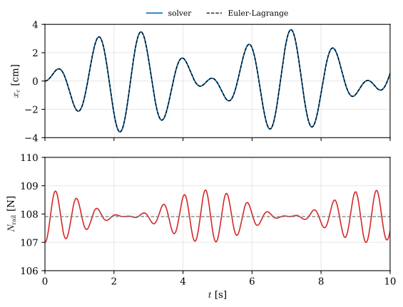
The pendulum on the cart of Rigid body kinetics and Euler-Lagrange (Figure 7.6.3) has two bodies and six coordinates. The cart slides on the rail without turning, \(y_c = 0\) and \(\varphi_c = 0\), and the bar is pinned at its end to the centre of the cart: four constraints, two degrees of freedom. The applied forces are gravity on both bodies and the spring force \(-kx_c\) on the cart. With \(M = 10\) kg, \(k = 270\) N/m, \(m = 1\) kg, \(L = 0.6\) m and the bar released at \(20^\circ\), we integrate ten seconds with \(\Delta t = 1\) ms and projection, and compare with the two Euler-Lagrange equations integrated with a fine step.

M_c, k_c, m_p, L_p = 10.0, 270.0, 1.0, 0.6
cart = Mechanism()
c_b = cart.body('c', M_c, 1.0)
p_b = cart.body('p', m_p, m_p*L_p**2/12)
cart.add(cart.bodies[c_b]['q'][1])                     # on the rail
cart.add(cart.bodies[c_b]['q'][2])                     # without turning
cart.pin(p_b, (-L_p/2, 0), c_b, (0, 0))                # the bar's end at the centre of the cart
cart.build()
f_cart = lambda q, qd, t_: np.array([-k_c*q[0], -M_c*g, 0, 0, -m_p*g, 0.0])
th0 = np.radians(20)
q0 = [0, 0, 0, L_p/2*np.sin(th0), -L_p/2*np.cos(th0), th0 - np.pi/2]
tc, Qc, QDc, LAMc = cart.simulate(q0, np.zeros(6), f_cart, T=10.0, dt=1e-3)
th_c = Qc[:, 5] + np.pi/2

def lagrange(T=10.0, dt=1e-5, every=100):
    x, th, v, w, out = 0.0, th0, 0.0, 0.0, []
    for i in range(int(T/dt)):
        if i % every == 0:
            out.append((x, th))
        a11, a12, a22 = M_c + m_p, m_p*L_p/2*np.cos(th), m_p*L_p**2/3
        b1, b2 = -k_c*x + m_p*L_p/2*np.sin(th)*w**2, -m_p*g*L_p/2*np.sin(th)
        det = a11*a22 - a12**2
        v += dt*(b1*a22 - a12*b2)/det
        w += dt*(a11*b2 - a12*b1)/det
        x += dt*v
        th += dt*w
    return np.array(out)

ref = lagrange()
n_cmp = min(len(ref), len(Qc))
dx_max = np.max(np.abs(Qc[:n_cmp, 0] - ref[:n_cmp, 0]))
dth_max = np.max(np.abs(th_c[:n_cmp] - ref[:n_cmp, 1]))
E_c = (M_c*QDc[:, 0]**2 + m_p*(QDc[:, 3]**2 + QDc[:, 4]**2) + m_p*L_p**2/12*QDc[:, 5]**2 + k_c*Qc[:, 0]**2)/2 \
      + m_p*g*Qc[:, 4]
drift_c = np.max(np.abs(E_c - E_c[0]))/(m_p*g*L_p/2*(1 - np.cos(th0)))
N_rail = -LAMc[:, 0]                                   # the rail's force on the cart, from y_c = 0

The differences from the Euler-Lagrange solution over ten seconds, the energy drift, and the range of the rail’s force on the cart are

fig, axes = plt.subplots(2, 1, figsize=(6, 4.6), sharex=True)
axes[0].plot(tc, 100*Qc[:, 0], color='C0', lw=1.4, label='solver')
axes[0].plot(np.arange(len(ref))*1e-3, 100*ref[:, 0], 'k--', lw=0.9, label='Euler-Lagrange')
axes[0].set_ylabel('$x_c$ [cm]'); axes[0].set_ylim(-4, 4)
axes[0].legend(loc='lower center', bbox_to_anchor=(0.5, 1.0), fontsize=8, ncol=2, frameon=False)
axes[1].plot(tc, N_rail, color='C3', lw=1.2)
axes[1].axhline((M_c + m_p)*g, color='0.5', ls='--', lw=1)
axes[1].set_ylabel(r'$N_{\mathrm{rail}}$ [N]'); axes[1].set_xlabel('$t$ [s]'); axes[1].set_ylim(106, 110)
for a in axes: a.grid(alpha=0.3); a.set_xlim(0, 10)
end_ticks(fig)
plt.tight_layout(); plt.show()

The solver and the two Euler-Lagrange equations give the same motion, and the solver also gives what Lagrange left out: the multiplier of \(y_c = 0\) is the force of the rail on the cart. It swings around the total weight, by about one newton either way, as the bar’s centre of mass rises and falls. Six coordinates and four constraints did the work of two well-chosen coordinates, without anyone choosing them.

Stiff systems and implicit integration

The explicit step above must resolve the fastest motion in the model. A vehicle model whose body rolls over a hill in seconds while a stiff bushing vibrates in milliseconds needs a time step set by the bushing, millions of steps for a few seconds of driving. Such a model is called stiff: the difficulty lies in the spread of time scales, not in the stiffness of any part.

Industrial solvers therefore integrate implicitly. The simplest implicit method, backward Euler, evaluates the equations at the unknown end of the step,

\[ \dot{\bm q}_{n+1} = \dot{\bm q}_n + \Delta t\,\ddot{\bm q}_{n+1} , \qquad \bm q_{n+1} = \bm q_n + \Delta t\,\dot{\bm q}_{n+1} , \]

and makes every step a nonlinear system for \(\bm Z = (\bm q_{n+1}, \dot{\bm q}_{n+1}, \bm\lambda_{n+1})\), the residual

\[ \bm R(\bm Z) = \begin{bmatrix} \bm M\dfrac{\dot{\bm q}_{n+1} - \dot{\bm q}_n}{\Delta t} + \bm J^\mathsf{T}(\bm q_{n+1})\bm\lambda_{n+1} - \bm f(\bm q_{n+1}, \dot{\bm q}_{n+1}) \\ \bm q_{n+1} - \bm q_n - \Delta t\,\dot{\bm q}_{n+1} \\ \bm C(\bm q_{n+1}, t_{n+1}) \end{bmatrix} = \bm 0 , \]

solved by Newton-Raphson within each step. The position constraints are part of the residual, so the positions satisfy them at every step without a separate projection. The velocity constraints are not, in this form; formulations that add them are offered by the industrial solvers. The price is a large linear system per Newton iteration, whose matrix holds the mass matrix, the constraint Jacobian and the derivatives of the forces. The reward is stability: the step can be as long as the slow motion allows, while the fast vibrations are damped out by the method.

Adams’ default integrator, GSTIFF, is of this kind: a backward differentiation formula that fits a polynomial through several past steps, and that changes its order between one and six and its step length during the run, by estimating its own error. It shortens the step through an impact and lengthens it again when the motion is smooth.

From here

The block system 7.10.4, a mass or stiffness matrix bordered by a constraint Jacobian and its transpose, is also how a finite element program enforces a prescribed displacement or a tied contact with Lagrange multipliers, and its multipliers are again the reaction forces. The penalty contact of Impulse, momentum and impact is the alternative: a stiff spring where the constraint would be, with no multiplier and a small violation of the constraint instead.

Further reading

The method of this chapter, body coordinates with constraint equations and multipliers, is treated in full by Nikravesh [1], by Haug [2], who works in the same Cartesian coordinates, and by García de Jalón and Bayo [3], who discuss the formulations and their efficiency in depth.