Code
aa = sp.Matrix([3, 2])
bb = sp.Matrix([1, 3])“The only way to learn mathematics is to do mathematics.”
— Paul R. Halmos, A Hilbert Space Problem Book, 1967
Some quantities are settled by one number, a length, a temperature, a mass. Such a quantity is a scalar. Others need a direction as well: the displacement from one corner of a room to another is not described by its length alone. A quantity with both a size and a direction is a vector.
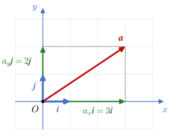
On squared paper a vector is a set of steps. From the origin \(O\) we take three steps along the unit arrow \(\bm i\) of the \(x\) axis and two along the unit arrow \(\bm j\) of the \(y\) axis. The arrow from \(O\) to the point where we stop is the vector \(\bm a\), and the two numbers stacked in brackets record the steps. Negative steps go the other way: \(\bm b\) is two steps back along \(x\) and three down along \(y\).
We draw a vector as an arrow. The arrow starts at its foot and ends at its tip; its length is the size of the vector and the arrow points in its direction. In print we write vectors in bold italic, \(\bm a\), \(\bm u\), \(\bm r\), and by hand with a bar under the letter, \(\underline a\), or an arrow over it, \(\vec a\). The length of \(\bm a\) is written \(|\bm a|\) or, when no confusion is possible, plain \(a\). The length is a scalar, never negative.
A vector of length one is a unit vector; we name unit vectors \(\bm e\) with an index that tells the direction, \(\bm e_a\) for the unit vector along \(\bm a\). The vector of length zero is the zero vector \(\bm 0\). It has no direction and must not be confused with the number \(0\), its length, \(|\bm 0| = 0\).
Drag the tip of \(\bm a\) and watch the two numbers of its column change with the steps.
Two vectors are equal, \(\bm a = \bm b\), when they have the same length and the same direction. Where the arrows are drawn plays no part: an arrow moved without turning or stretching it is the same vector. All the arrows in the video are one and the same vector.
This freedom to move arrows is what makes the drawings of the next sections possible.
To add \(\bm b\) to \(\bm a\) we place the foot of \(\bm b\) at the tip of \(\bm a\). The sum \(\bm a + \bm b\) is the arrow from the foot of \(\bm a\) to the tip of \(\bm b\). Adding vectors is travelling a path: walk along \(\bm a\), then along \(\bm b\), and the sum is the shortcut from the start to the end.
Walking along \(\bm b\) first and \(\bm a\) second ends at the same point, so \(\bm a + \bm b = \bm b + \bm a\). The two paths are the sides of a parallelogram and the sum is its diagonal. With three vectors the brackets do not matter either, \((\bm a + \bm b) + \bm c = \bm a + (\bm b + \bm c)\): the path is the same.
The vector \(-\bm b\) has the length of \(\bm b\) and the opposite direction: the same arrow walked backwards. Subtracting is adding the reversed vector,
\[ \bm a - \bm b = \bm a + (-\bm b), \]
so we walk along \(\bm a\) and then backwards along \(\bm b\).
A vector minus itself is the walk there and back, \(\bm a - \bm a = \bm 0\).
A number \(s\) times a vector \(\bm a\) is the vector \(s\bm a\) with the length \(|s|\,|\bm a|\), on the same line as \(\bm a\). For \(s > 0\) it points the same way as \(\bm a\), for \(s < 0\) the opposite way, and \((-1)\bm a = -\bm a\). Scaling keeps a vector on its line, which gives the test for two vectors being parallel:
\[ \bm a \parallel \bm b \quad\Longleftrightarrow\quad \bm a = s\,\bm b \ \text{ for some number } s \tag{3.5.1}\]
Parallel vectors lie on the same line, or on parallel lines, and point the same way or opposite ways. The zero vector is \(0\,\bm b\) and so counts as parallel to every vector. Together with the test for perpendicular vectors in Chapter 3.6, 3.5.1 is the tool we reach for most often when we model with vectors.
Arrows on paper are fine for thinking, but to compute we need numbers. We fix a point, the origin \(O\), and three mutually perpendicular unit vectors \(\bm i\), \(\bm j\) and \(\bm k\) along the \(x\), \(y\) and \(z\) axes, arranged as a right-handed system. These are the basis vectors. We start in the plane, with \(\bm i\) and \(\bm j\) alone.
Every vector in the plane is the sum of a vector along \(\bm i\) and a vector along \(\bm j\),
\[ \bm a = a_x\bm i + a_y\bm j. \]
The two vectors \(a_x\bm i\) and \(a_y\bm j\) are the composants of \(\bm a\), vectors themselves. The numbers \(a_x\) and \(a_y\) are its components, scalars, the amounts of each basis vector we need. Figure 3.5.1 shows \(\bm a = 3\bm i + 2\bm j\): three steps along \(x\) and two along \(y\).
We collect the components in a column, the column vector
\[ \bm a = \begin{bmatrix} a_x \\ a_y \end{bmatrix} = \begin{bmatrix} 3 \\ 2 \end{bmatrix}. \]
In running text the column takes much room, so we often write it lying down and mark it with the transpose, \(\bm a = [3, 2]^\mathsf{T}\).
In space the third basis vector \(\bm k\) joins in,
\[ \bm a = a_x\bm i + a_y\bm j + a_z\bm k = \begin{bmatrix} a_x \\ a_y \\ a_z \end{bmatrix}, \qquad \bm i = \begin{bmatrix} 1 \\ 0 \\ 0 \end{bmatrix},\quad \bm j = \begin{bmatrix} 0 \\ 1 \\ 0 \end{bmatrix},\quad \bm k = \begin{bmatrix} 0 \\ 0 \\ 1 \end{bmatrix}. \]
Grant Sanderson opens his series Essence of linear algebra with the same two views of a vector, the arrow and the column of components, and shows addition and scaling in both.
Addition and scaling now become arithmetic on the components, row by row:
\[ \bm a + \bm b = \begin{bmatrix} a_x + b_x \\ a_y + b_y \\ a_z + b_z \end{bmatrix}, \qquad \bm a - \bm b = \begin{bmatrix} a_x - b_x \\ a_y - b_y \\ a_z - b_z \end{bmatrix}, \qquad s\bm a = \begin{bmatrix} s a_x \\ s a_y \\ s a_z \end{bmatrix}. \]
Two vectors are equal when all their components are equal. The path of the video on addition is the same statement drawn: the \(x\) steps add up and the \(y\) steps add up.
In SymPy a column vector is a sp.Matrix built from a list, and +, - and multiplication by a number act row by row. We name vectors with a doubled letter, aa for \(\bm a\), so that the plain letter stays free for its length.
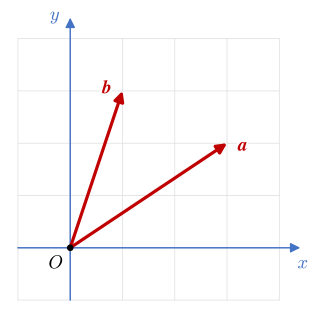
For \(\bm a = [3, 2]^\mathsf{T}\) and \(\bm b = [1, 3]^\mathsf{T}\) in Figure 3.5.2, find \(\bm a + \bm b\), \(\bm a - \bm b\) and \(2\bm a - 3\bm b\).
Each result is a row-by-row calculation, \(\bm a + \bm b = [3 + 1, 2 + 3]^\mathsf{T}\) and so on. In SymPy:
aa = sp.Matrix([3, 2])
bb = sp.Matrix([1, 3])The three results are
\[ \bm a + \bm b = \left[\begin{matrix}4\\5\end{matrix}\right],\quad \bm a - \bm b = \left[\begin{matrix}2\\-1\end{matrix}\right],\quad 2\bm a - 3\bm b = \left[\begin{matrix}3\\-5\end{matrix}\right] \]
Drawn tip to tail, \(\bm a + \bm b\) ends four steps right and five up from the origin, which is the column \([4, 5]^\mathsf{T}\).
A point \(P\) is a place, given by its coordinates, which we write in a row with round brackets, \(P = (P_x, P_y, P_z)\). A point is not a vector: it has no length and no direction, and adding two places means nothing. The link between them is the position vector \(\bm r_{OP}\), the arrow from the origin \(O\) to \(P\). Its components are the coordinates of the point, written as a column,
\[ \bm r_{OP} = \overrightarrow{OP} = \begin{bmatrix} P_x \\ P_y \\ P_z \end{bmatrix}. \]
The point \(A = (1, 2)\) and the vector \(\bm a = [1, 2]^\mathsf{T}\) share their two numbers and nothing else. \(A\) is one place on the grid. \(\bm a\) is a step, one along \(x\) and two along \(y\), that can start anywhere; only when it starts at the origin does its tip land on \(A\), and then \(\bm a = \bm r_{OA}\). The brackets keep the two apart: round for points, square for vectors.
The vector from a point \(A\) to a point \(B\) follows from a walk: from \(A\) back to the origin, which is \(-\bm r_{OA}\), and from the origin out to \(B\), which is \(\bm r_{OB}\),
\[ \bm r_{AB} = \bm r_{OB} - \bm r_{OA} \tag{3.5.2}\]
head minus foot
The order matters: the point the arrow points to comes first. Swapping them gives \(\bm r_{BA} = -\bm r_{AB}\), the same arrow reversed. When someone writes \(B - A\) for two points, the position vectors are meant.
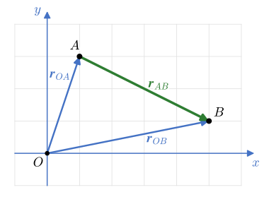
Find the vector from \(A(1, 3)\) to \(B(5, 1)\) in Figure 3.5.3.
The position vectors carry the coordinates of the points, and 3.5.2 subtracts the foot from the head:
rr_OA = sp.Matrix([1, 3])
rr_OB = sp.Matrix([5, 1])
rr_AB = rr_OB - rr_OA
which gives
\[ \bm r_{AB} = \left[\begin{matrix}5\\1\end{matrix}\right] - \left[\begin{matrix}1\\3\end{matrix}\right] = \left[\begin{matrix}4\\-2\end{matrix}\right] \]
Four steps right and two down, as the arrow in Figure 3.5.3 shows.
Practise the subtraction below. Type the two components of \(\bm r_{AB}\); the arrow is drawn from \(A\) with the steps you enter, so a wrong answer shows where it misses \(B\).
The components of a vector in the plane are the legs of a right triangle and the vector is its hypotenuse, so Pythagoras gives the length. In space the theorem is used twice, once in the \(xy\) plane and once more upwards, and
\[ |\bm a| = \sqrt{a_x^2 + a_y^2 + a_z^2}. \tag{3.5.3}\]
The squares make every term positive, so a minus sign in a component never reduces the length: \(|[1, -2, 3]^\mathsf{T}| = \sqrt{1 + 4 + 9} = \sqrt{14}\). Only the zero vector has length zero, since all three squares must vanish. In SymPy, aa.norm() computes 3.5.3.
Dividing a vector by its length keeps its direction and makes its length one, so
\[ \bm e_a = \frac{\bm a}{|\bm a|} \tag{3.5.4}\]
is the unit vector along \(\bm a\). The division is shorthand for multiplying by the number \(1/|\bm a|\). Read backwards, 3.5.4 splits every vector into two parts.
Every vector is its length times the unit vector in its direction,
\[ \bm a = |\bm a|\,\bm e_a . \]
The length is a number with the units of the quantity; the unit vector is a pure direction, without units. To build a vector we find these two parts separately and multiply them.
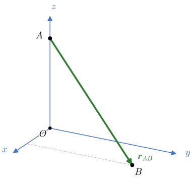
For the points \(A(0, 0, 4)\) and \(B(2, 5, 0)\) in Figure 3.5.4, find the vector \(\bm r_{AB}\), its length and the unit vector along it. Then find the vector \(\bm c\) of length \(5\) that points from \(A\) towards \(B\).
The vector between the points is head minus foot, and its length and unit vector follow from 3.5.3 and 3.5.4:
rr_OA = sp.Matrix([0, 0, 4])
rr_OB = sp.Matrix([2, 5, 0])
rr_AB = rr_OB - rr_OA
r_AB = rr_AB.norm()
ee_AB = rr_AB/r_AB
The vector, its length and its direction are
\[ \bm r_{AB} = \left[\begin{matrix}2\\5\\-4\end{matrix}\right],\quad |\bm r_{AB}| = 3 \sqrt{5},\quad \bm e_{AB} = \left[\begin{matrix}\dfrac{2 \sqrt{5}}{15}\\\dfrac{\sqrt{5}}{3}\\- \dfrac{4 \sqrt{5}}{15}\end{matrix}\right] \]
The vector \(\bm c\) has the length \(5\) and the direction \(\bm e_{AB}\), so it is the product of the two:
cc = 5*ee_AB\[ \bm c = 5\,\bm e_{AB} = \left[\begin{matrix}\dfrac{2 \sqrt{5}}{3}\\\dfrac{5 \sqrt{5}}{3}\\- \dfrac{4 \sqrt{5}}{3}\end{matrix}\right],\quad |\bm c| = 5 \]
The check \(|\bm c| = 5\) confirms that the unit vector really had length one.
Practise the length and the unit vector between two points below. The fields accept expressions such as sqrt(29) and 2/sqrt(29).
Components come from right triangles. In the right triangle of Figure 3.5.5, the side next to the angle \(\alpha\) is the adjacent side, the side across from it is the opposite side, and the longest side, across from the right angle, is the hypotenuse. Sine, cosine and tangent are ratios of these sides,
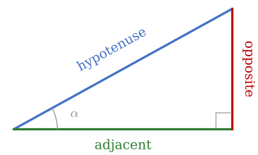
\[ \sin\alpha = \frac{\text{opposite}}{\text{hypotenuse}}, \qquad \cos\alpha = \frac{\text{adjacent}}{\text{hypotenuse}}, \qquad \tan\alpha = \frac{\text{opposite}}{\text{adjacent}}. \tag{3.5.5}\]
To find the components of a vector, we look for a right triangle with the vector as its hypotenuse, decide which leg is adjacent to the given angle and which is opposite, and multiply the length by the cosine or the sine. The triangle gives only the lengths of the legs, so the sign of each component is read from the figure. Every problem brings a new triangle, the given angle may sit against the \(x\) axis in one problem and against the \(y\) axis in the next, and every sign is set by eye. This is tedious, and a wrong sign is easy to miss. The unit circle replaces all these triangles with a single one.
In the plane, a unit vector is fixed by one angle. Measure the angle \(\theta\) from the positive \(x\) axis, counter-clockwise positive. The unit vector at that angle has its tip on the circle of radius one around the origin, the unit circle. The right triangle under it has the hypotenuse one, so by 3.5.5 its legs are \(\cos\theta\) along \(x\) and \(\sin\theta\) along \(y\). The legs are the components:
\[ \bm e(\theta) = \begin{bmatrix} \cos\theta \\ \sin\theta \end{bmatrix} \tag{3.5.6}\]
cosine in the \(x\) component, sine in the \(y\) component
Drag the tip of \(\bm e\) around the circle. Near the standard angles it snaps into place and shows the exact values of the components, the angle in degrees and in radians.
As \(\theta\) grows past \(90°\) the cosine turns negative, and the arrow points to the left; past \(180°\) the sine turns negative too. The signs of the components follow the quadrant by themselves, with no rule to remember. Turning the vector at a steady rate and following its two components over time draws the cosine and the sine as waves.
With 3.5.6 and the two parts of a vector, a vector of length \(a\) at the angle \(\theta\) from the positive \(x\) axis is
\[ \bm a = a \begin{bmatrix} \cos\theta \\ \sin\theta \end{bmatrix}. \tag{3.5.7}\]
Drag the tip of \(\bm a\) below and watch the components, the length and the angle. The unit circle option draws \(\bm e_a\) and its two legs.
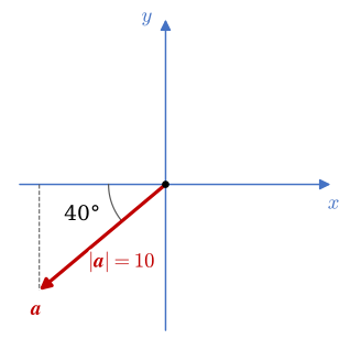
The vector \(\bm a\) in Figure 3.5.6 has the length \(10\) and points \(40°\) below the negative \(x\) axis. Find its components, first with a triangle and then with the unit circle.
The triangle has \(\bm a\) as its hypotenuse and the \(40°\) angle at the origin. The adjacent leg lies on the \(x\) axis and the opposite leg is the dashed line, so by 3.5.5 the legs have the lengths \(10\cos 40°\) and \(10\sin 40°\). The figure shows that both legs point in the negative directions, and we add the minus signs by hand:
\[ \bm a = \begin{bmatrix} -10\cos 40° \\ -10\sin 40° \end{bmatrix}. \]
The unit circle needs the angle from the positive \(x\) axis. Half a turn reaches the negative \(x\) axis and \(40°\) more reaches \(\bm a\), so \(\theta = 180° + 40° = 220°\), as in Figure 3.5.7.
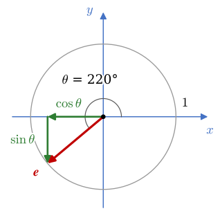
3.5.7 then gives the components, signs included:
theta = sp.rad(220)
aa = 10*sp.Matrix([sp.cos(theta), sp.sin(theta)])
The components, exact and to three digits, are
\[ \bm a = 10\begin{bmatrix}\cos 220^\circ \\ \sin 220^\circ\end{bmatrix} = \left[\begin{matrix}- 10 \cos{\left(\dfrac{2 \pi}{9} \right)}\\- 10 \sin{\left(\dfrac{2 \pi}{9} \right)}\end{matrix}\right] \approx \left[\begin{matrix}-7.66\\-6.43\end{matrix}\right] \]
SymPy rewrites \(\cos 220°\) as \(-\cos 40°\) by itself, with the angle in radians, \(40° = 2\pi/9\). Both ways give the same vector, but the unit circle needed no triangle and no look at the figure for the signs, only the angle from the positive \(x\) axis.
Every problem below gives a vector by its length and an angle measured from some axis, in either sense. Turn the angle into \(\theta\) from the positive \(x\) axis, then write \(a_x = a\cos\theta\) and \(a_y = a\sin\theta\). The answer fields accept numbers and expressions such as 200*cos(180-35), with angles in degrees. The worked answer is blurred until the pointer rests on it. Solve until the conversion needs no thought.
A drawing that gives points, lengths or slopes already holds every direction we need. A common habit throws that away: first an angle is computed from the geometry with \(\arctan\), \(\arcsin\) or \(\arccos\), and then the angle is fed straight back into \(\cos\) and \(\sin\) to get the components. The round trip gains nothing. The cosine and sine of an angle in a right triangle are ratios of its sides, and the geometry gave us those sides before any angle existed. What the round trip adds is the step out through the inverse function, and that is where the errors enter.
The direction is in the geometry, \(\bm e_{AB} = \bm r_{AB}/|\bm r_{AB}|\). Never compute an angle only to take its cosine and sine.
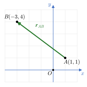
Find the unit vector that points from \(A(1, 1)\) to \(B(-3, 4)\) in Figure 3.5.8, once through an angle and once directly.
Head minus foot gives \(\bm r_{AB} = [-4, 3]^\mathsf{T}\), four steps left and three up, and its length is \(5\). The detour reads the slope \(3/(-4)\) as \(\tan\theta\), asks the calculator for the angle and builds the unit vector from it:
rr_AB = sp.Matrix([-3, 4]) - sp.Matrix([1, 1])
theta = sp.atan(sp.Rational(3, -4))
ee_detour = sp.Matrix([sp.cos(theta), sp.sin(theta)])
The angle and the unit vector it leads to are
\[ \theta = \arctan\frac{3}{-4} \approx -36.87^\circ,\quad \bm e = \left[\begin{matrix}\dfrac{4}{5}\\- \dfrac{3}{5}\end{matrix}\right] \]
This arrow points down and to the right, from \(B\) back towards \(A\). The calculator is not at fault: \(\arctan\) returns an angle between \(-90°\) and \(90°\), and the quotient \(3/(-4)\) is the same as \((-3)/4\), so it cannot know that we travel to the left. The direct route never leaves the vectors:
ee_AB = rr_AB/rr_AB.norm()\[ \bm e_{AB} = \frac{\bm r_{AB}}{|\bm r_{AB}|} = \left[\begin{matrix}- \dfrac{4}{5}\\\dfrac{3}{5}\end{matrix}\right] \]
Head minus foot, divided by the length: one line, no angle, and the right sign in every quadrant. Had \(B\) lain to the right of \(A\), the detour would have given the right answer, and that is the worse outcome, since the habit then seems to work until the day it does not.
The inverse functions all share this flaw. Each returns one angle out of the several that have the same tangent, sine or cosine. For \(\arctan\) the lost information is the quadrant: the quotient \(a_y/a_x\) is the same for \(\bm a\) and \(-\bm a\).
The sine rule loses a triangle the same way. It delivers \(\sin B\), and \(\arcsin\) returns an angle between \(-90°\) and \(90°\), while a triangle can have \(B\) or \(180° - B\) with the same sine. Given two sides and the angle opposite one of them, two triangles can fit, and the sine rule finds only one.
Going the other way is safe. When a drawing gives an angle, \(\cos\theta\) and \(\sin\theta\) have exactly one value each, so turning a given angle into components with 3.5.7, as in the practice above, cannot go wrong once \(\theta\) is measured from the positive \(x\) axis. The danger lies only on the way back, from geometry to an angle.
Sometimes the angle itself is the answer: the angle a vector makes with the \(x\) axis, or the angle between two vectors. Then we compute it from the vectors, with \(\operatorname{atan2}(a_y, a_x)\), which keeps the signs of both components and returns the right angle in every quadrant, or with the dot product of Chapter 3.6, whose \(\arccos\) works in its safe range between \(0°\) and \(180°\). The cosines of the angles between a vector and the three axes, sometimes called direction cosines, are nothing more than the components of its unit vector, so the unit vector serves directly.
The same holds for unknowns. When a model needs a direction that is not known in advance, an unknown unit vector or unknown components keep the equations polynomial and valid in every quadrant, while an unknown angle brings in trigonometric equations with several solutions in each period.
Given points or lengths, build the direction from them, \(\bm e_{AB} = \bm r_{AB}/|\bm r_{AB}|\). Given an angle, convert it once with cosine in \(x\) and sine in \(y\). Compute an angle only when the angle is the answer, and then with atan2 or the dot product.