15.2 Linear static analysis in SolidWorks Simulation
SolidWorks Simulation is the finite element module inside the CAD program, so the part we have drawn is the part we analyse, and a change of a dimension reaches the result in a few seconds. The price is that the program decides a great deal for us. It meshes, it chooses the element type, and it solves without asking, so a model that runs is not yet a model we can trust. This chapter sets up three linear static studies of flat plates and checks every one of them, against the stress concentration factor of a hole, against \(\sigma = F/A\) and against equilibrium. The theory behind each step is in Chapter 8.21.
Starting a study
Simulation is an add-in. If the Simulation tab is missing, open Tools, Add-Ins and tick SOLIDWORKS Simulation, and tick the Start Up column too if it should load with every session, at the cost of a slower start. Save the part on a local disk before the study is created. Simulation writes many result files next to the part, and a folder synchronised by OneDrive or Dropbox locks some of them while they are written, which makes the solver complain or fail.
On the Simulation tab, New Study opens a list of analysis types. We choose Static. The study appears as a tree below the feature tree, and we work through it from the top: a material, the fixtures, the external loads, the mesh, and finally Run This Study, after which the Results folder holds plots of stress, displacement and strain. The same commands sit on the ribbon from left to right.
Example 1: A steel plate with two holes
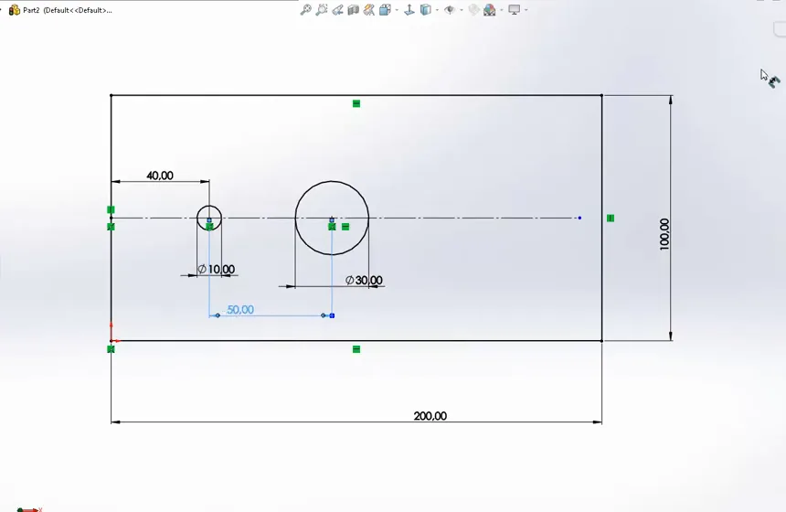
A steel plate of \(200 \times 100\) mm and thickness \(t = 8\) mm has two holes on its centre line, of diameter \(10\) mm at \(40\) mm from the left edge and of diameter \(30\) mm at \(50\) mm further on (Figure 15.2.1). The right edge carries a tensile force of \(F = 32\) kN and the left edge is held. We want the largest stress in the plate.
Material
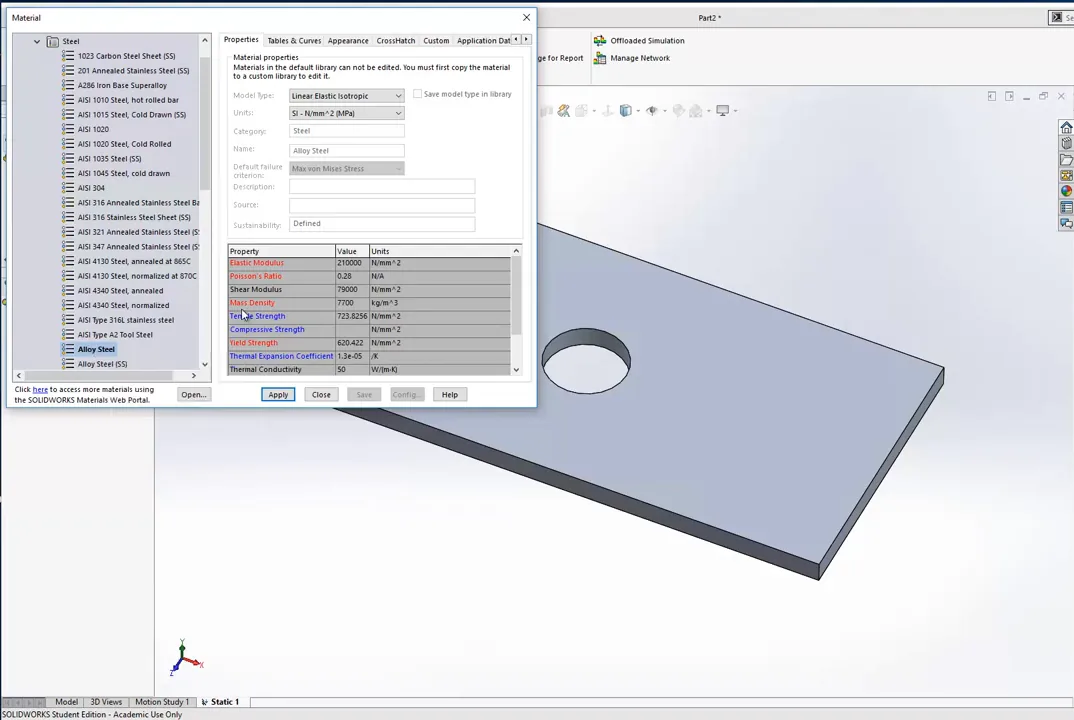
Apply Material opens the material library with Alloy Steel selected (Figure 15.2.2). Set Units to SI - N/mm^2 (MPa), so that every stress in the study is in MPa. The properties drawn in red are those the chosen analysis uses. A linear static analysis needs only the elastic modulus \(E\) and Poisson’s ratio \(\nu\). The density enters only with a gravity load, and the yield strength is used only by a factor of safety plot. We read the strength from the data sheet of the real material and compare it with the result ourselves.
Load and fixture
External Loads, Force, on the right end face, with Normal direction, Reverse direction ticked so that the force pulls, and \(32\,000\) N. Fixtures, Fixed Geometry, on the left end face.
A Fixed Geometry face cannot move in any direction, a condition stricter than any real clamp: the plate wants to contract sideways under tension, by Poisson’s ratio, and the fixed face forbids it. The stresses near that face are therefore wrong, and we do not read them. Section 15.2.3 shows how large the error is and how to remove it. Away from the fixture, by Saint-Venant’s principle, the fixed face is a fair model of a plate welded or clamped along its edge.
Running and reading the result
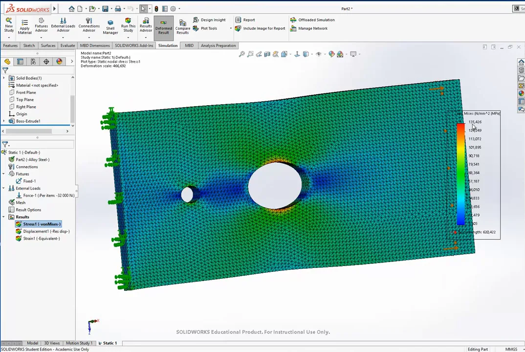
Run This Study meshes with the default settings and solves within seconds. The von Mises plot is the first result. Two settings make it readable. Right-click the plot, Edit Definition, and set the units to MPa; in Chart Options, set the number format to floating. The deformed shape is drawn with an automatic scale factor, here several hundred, because the true deformation of a steel plate this thick is invisible. Set the Deformed Shape to True scale to see the plate as it is, and back to Automatic to see the trend, with the plate stretched and narrowed beside the holes.
Figure 15.2.3 shows the stress on the finest mesh of the next section. The peak lies at the top and bottom of the large hole, on the diameter perpendicular to the load.
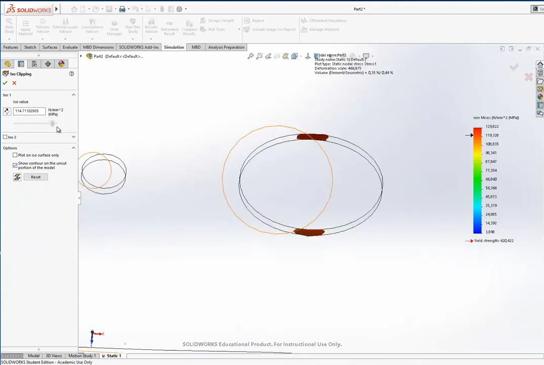
The Plot Tools give three ways to find where the stress is largest. Probe reports the stress at the point we click. Section Clipping cuts the part with a plane we can move, so that we see the stress inside the material. Iso Clipping hides every part of the model below a stress level we choose with a slider (Figure 15.2.4), and as the level rises, only the regions with the highest stress remain. Show max annotation, in Chart Options, marks the peak with a label. It is quick but tells us nothing about how large the region of high stress is.
Refining the mesh
The default mesh gives a peak of \(130\) MPa. To refine it, right-click Mesh, Create Mesh, and lower the global element size. A size of \(4\) mm puts two elements through the \(8\) mm thickness, and a size of \(2\) mm takes the peak to \(135\) MPa. The second refinement already gives about half a million degrees of freedom, so the stiffness matrix the solver factorises has half a million rows, and the solution takes noticeably longer. Since the peak changed by about \(4~\%\) from the default mesh and the refined meshes agree, the result has converged in the sense of Mesh convergence.
Checking the peak by hand
The net section through the large hole is \((w - d)t = (100 - 30) \cdot 8 = 560~\text{mm}^2\), so the nominal stress there is
\[ \sigma_{\text{nom}} = \frac{F}{(w - d)t} = \frac{32\,000}{560} = 57.1~\text{MPa} . \]
With \(d/w = 0.3\), 8.4.2 gives \(K_t = 2.35\), and the peak is \(K_t\sigma_{\text{nom}} = 134\) MPa. SolidWorks gives \(135\) MPa. For the small hole, \(d/w = 0.1\) gives \(K_t = 2.72\), \(\sigma_{\text{nom}} = 32\,000/(90 \cdot 8) = 44.4\) MPa and a peak of \(121\) MPa, the value the probe reports there. The chart treats each hole as alone in a long strip. Moving the holes towards each other in the sketch and solving again shows how far apart they must be before they stop interacting, a question no chart answers.
Example 2: Checking the fixtures on a plain plate
Before we trust a study, we solve one whose answer we know. A plate of \(200 \times 100\) mm and thickness \(10\) mm without holes, pulled with \(F = 1000\) N, carries
\[ \sigma = \frac{F}{A} = \frac{1000}{100 \cdot 10} = 1~\text{MPa} \]
everywhere, and lengthens by
\[ \delta = \frac{FL}{EA} = \frac{1000 \cdot 200}{210\,000 \cdot 1000} = 9.5 \cdot 10^{-4}~\text{mm} . \]
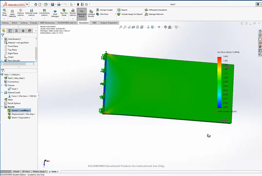
With the left face fixed as in Example 1, the von Mises plot reads \(1.00\) MPa over most of the plate and \(1.44\) MPa at the corners of the fixed face (Figure 15.2.5). The fixed face holds the plate at its original width and thickness while the rest of it contracts, and the restraint creates stresses that the real plate does not have.
The plate needs supports that stop it moving as a rigid body and nothing more, the condition discussed in Boundary conditions. A Roller/Slider fixture on the left face stops it moving along the load and lets the face slide freely in its own plane, so that the plate can contract. That alone leaves the plate free to slide and rotate in the plane of the face, and the solver either refuses or returns a solution that depends on round-off. Fixed Geometry on two vertices of the left face removes the remaining rigid body motion. The stress is now \(1.00\) MPa everywhere, apart from rounding in the last digit.
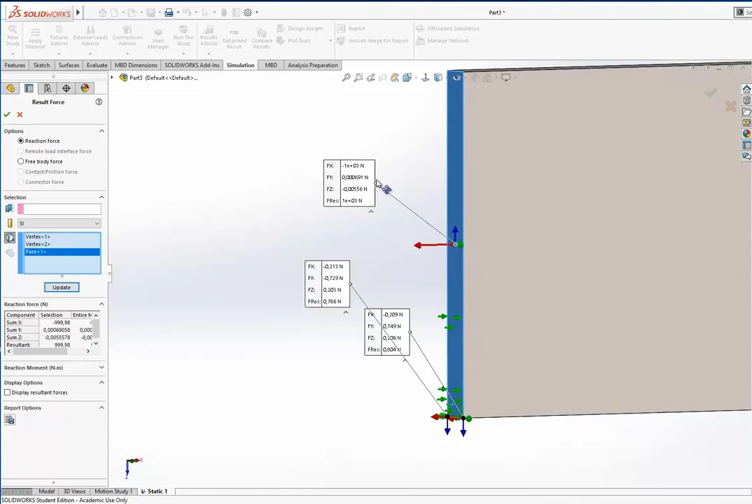
The reaction forces tell us whether the supports do only what we intended. Right-click Results, List Result Force, select the face and the two vertices, and Update (Figure 15.2.6). The face carries \(1000\) N in the direction of the load, so the plate is in equilibrium. Each vertex carries less than \(1\) N, the small force needed to hold the thickness contraction between the two fixed points. A single fixed vertex together with a restraint of one direction on a second vertex would remove even that. The displacement plot gives the elongation of \(9.5 \cdot 10^{-4}\) mm computed above.
Example 3: An aluminium plate with an offset hole
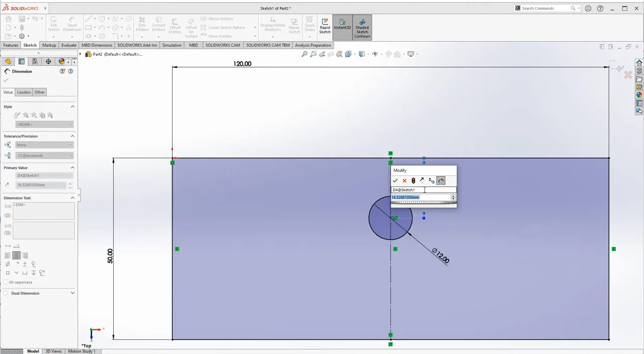
A plate of \(120 \times 50\) mm and thickness \(t = 3\) mm, in the aluminium alloy 6063-T6, has a hole of diameter \(12\) mm on its vertical centre line, \(16\) mm from the top edge (Figure 15.2.7). The left edge is fixed and the right edge carries \(F = 1000\) N in tension. The question can be posed two ways. How large a load can this design carry? Or, if the plate must carry a given load, for instance because a pipe passes through the hole, how large may the hole be and where may it go?
Material
6063-T6 is in the Aluminium Alloys folder of the library. All the aluminium alloys there have \(E \approx 69\) GPa, about a third of the value for steel, and the heat treatments differ only in strength: the yield strength of 6063 ranges from below \(50\) MPa annealed to \(215\) MPa in the T6 temper. The elastic modulus of a metal hardly depends on alloy or treatment, so the stresses of a linear study do not depend on which aluminium we pick. Only the comparison with the strength does.
The first result and where to read it
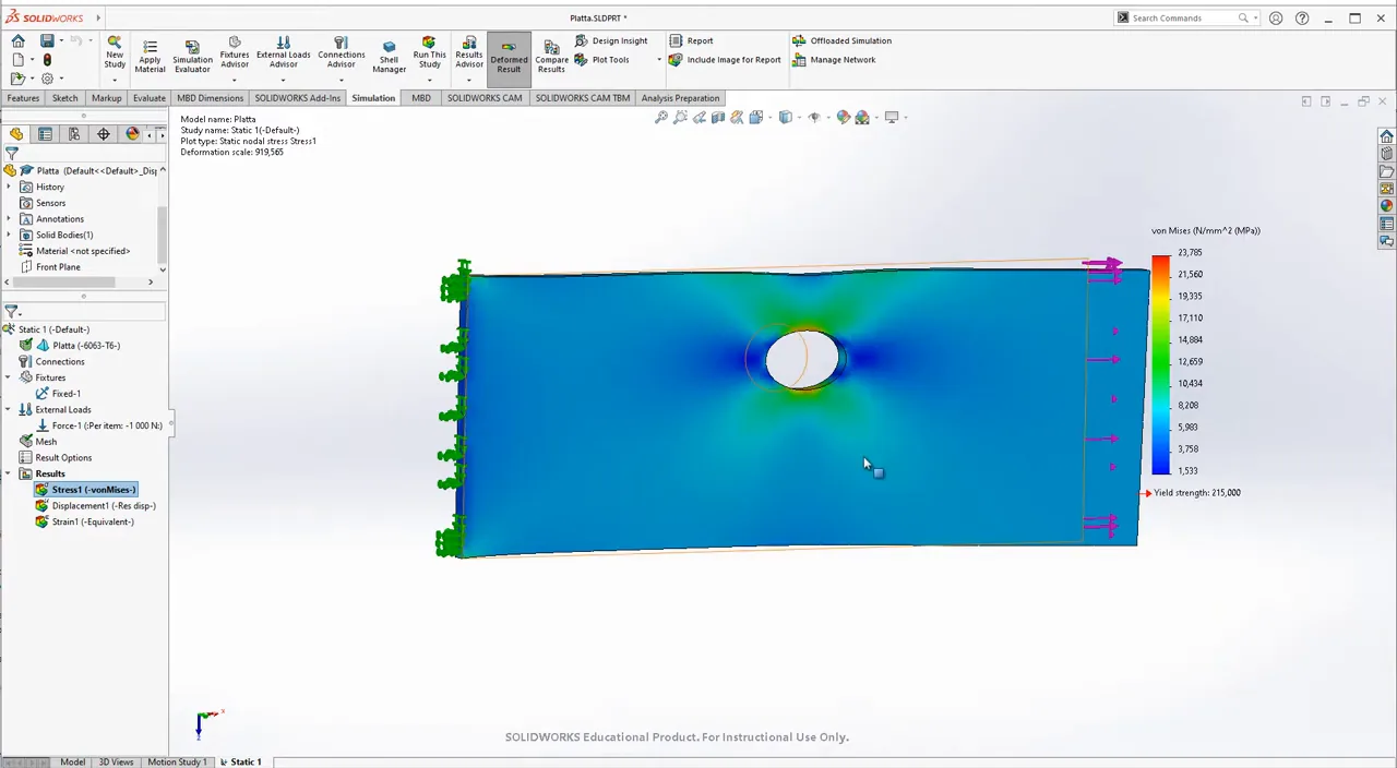
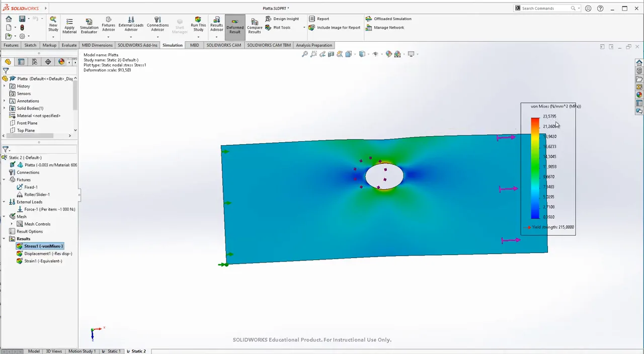
With the default mesh, the peak von Mises stress is \(23.8\) MPa, at the edge of the hole on the side of the narrow ligament (Figure 15.2.8). Against a yield strength of \(215\) MPa the plate can carry about nine times the load.
The fixture on the left edge is the same idealisation as in Example 1. The real plate is welded, bolted or clamped there, and how it is held decides the stresses near that edge. The model reports about \(10\) MPa in the top left corner, and that number means nothing, since it depends on a support we did not model. In many studies the highest stress of the whole part appears at a fixture or a load. We read the stresses in the region the question is about, here the hole, at a distance from the supports.
Checking the peak by hand
For a centred hole, \(d/w = 12/50 = 0.24\) gives \(K_t = 2.44\) by 8.4.2, and with \(\sigma_{\text{nom}} = 1000/((50 - 12) \cdot 3) = 8.8\) MPa the peak would be \(21.4\) MPa. Our hole is off centre. The ligament above it is \(10\) mm wide and the one below \(28\) mm, so the narrow ligament takes more than its share of the force, and the computed \(23.8\) MPa, about \(10~\%\) above the centred value, has the expected sign and size.
Mesh control
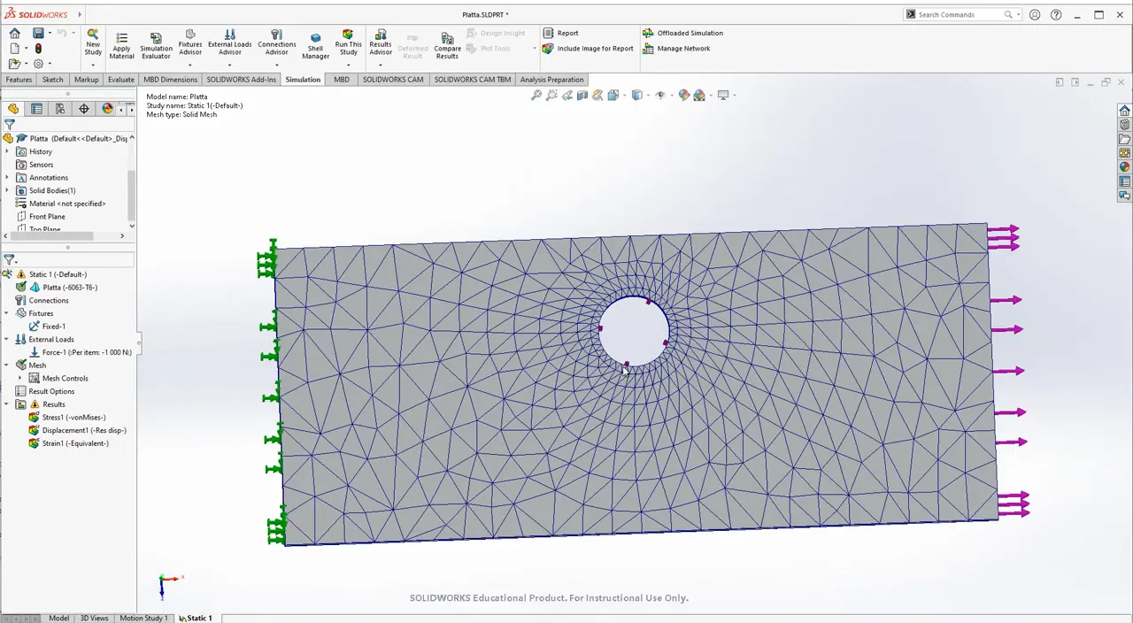
A uniformly fine mesh is wasted on the regions we do not read. Create Mesh with a global size of \(5\) mm, then right-click Mesh, Apply Mesh Control, select the face of the hole and set \(1\) mm there. The mesh is coarse along the edges and fine around the hole (Figure 15.2.9), and the peak becomes \(23.3\) MPa. A change of \(2~\%\) is negligible here. In other studies a local refinement changes the answer substantially, so we always make at least one.
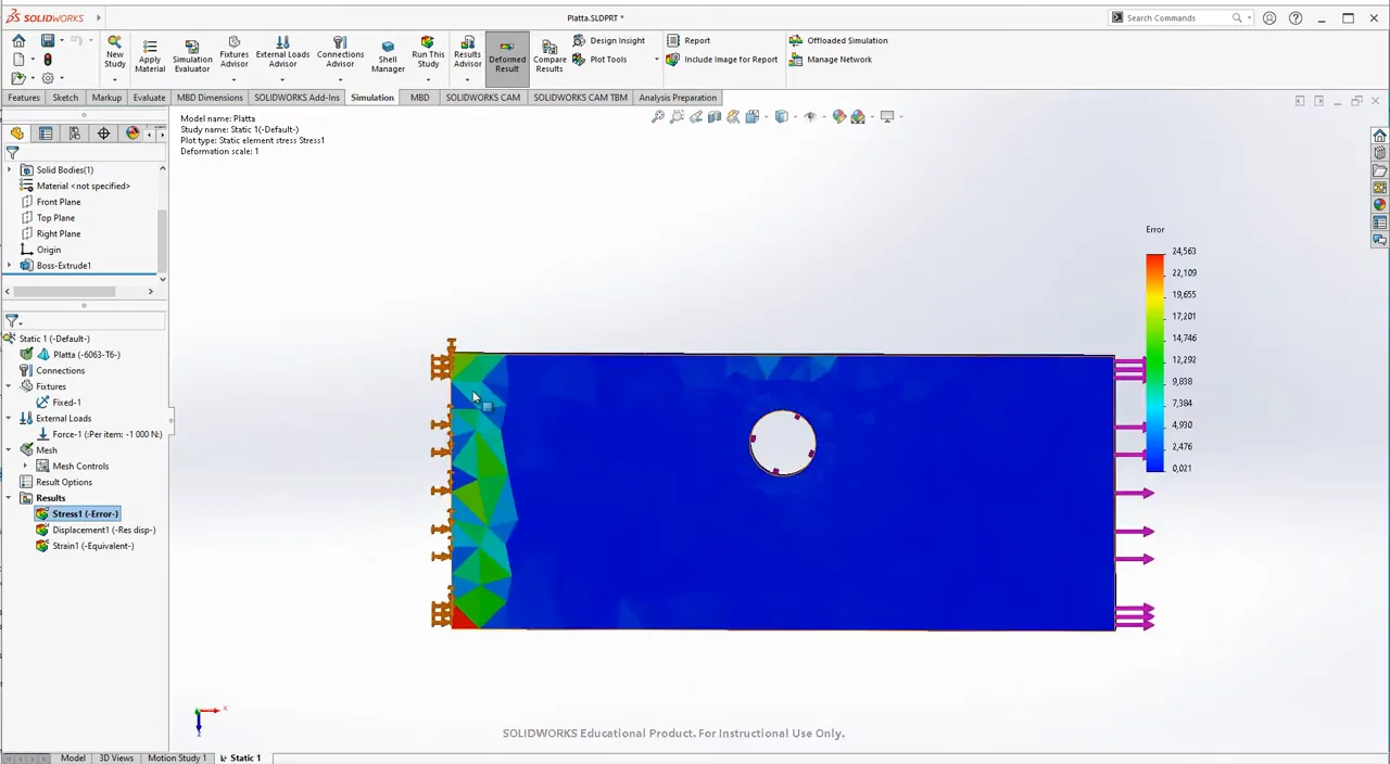
Two plots show whether a mesh resolves the stress. In Edit Definition, Advanced Options, switch from node values to element values. Each element is then drawn in one colour, the stress at its own integration points, without the averaging that smooths the default plot. Where neighbouring elements differ much, from \(17\) to \(20\) MPa next to the hole on the default mesh, the mesh is coarse for the gradient it has to represent. The second plot replaces von Mises by the energy norm error, an estimate of the discretisation error of each element (Figure 15.2.10). Its scale is relative, and here it is largest at the fixed edge and not at the hole, so the mesh where we read the result is adequate. The decisive test remains a refinement: refine, solve again and see whether the peak changes by more than a few percent.
Which stress to plot
Von Mises combines the six components of the stress tensor into one number, the equivalent stress of Yield criteria, which we compare with the yield strength. Edit Definition offers the components themselves. Here SX, the normal stress along the load, is close to von Mises, since the plate is mostly in uniaxial tension, and SY, SZ and the shear stresses are small. The principal stresses P1, P2 and P3 are the normal stresses in the directions where the shear stresses vanish. P1, the largest, shows where the material is pulled apart, and a negative P3 shows where it is compressed, here at the left and right of the hole, where the lines of force bend inwards.
The strain plot answers whether the linear model applies at all. The equivalent strain is of order \(\varepsilon = \sigma/E = 23/69\,000 = 3 \cdot 10^{-4}\), far inside the linear part of the tensile curve of Material properties. Were the strains beyond the yield strain, the stresses of a linear study would be fiction, since the material would have yielded long before. If the displacements become large, SolidWorks warns and offers a large displacement solution, which we meet in Chapter 15.3.
The same plate in plane stress
The plate is thin and loaded in its plane, the case of plane stress. A new Static study with Use 2D Simplification offers plane stress, plane strain and axisymmetric models. Choose Plane stress, select the face of the plate as the section and enter the thickness, \(3\) mm. The model is now a surface meshed with triangles. A fixed vertex at the bottom left corner and a Roller/Slider on the left edge hold it, so that the plate can contract across its width (Figure 15.2.11).
With a global size of \(5\) mm and a mesh control of \(0.7\) mm at the hole, the 2D model has \(2428\) nodes and \(1152\) triangles against \(6153\) nodes and \(3153\) tetrahedra for the 3D model, and still the finer elements at the hole. Right-click the result, Solver Messages, for the size of the problem: \(4854\) degrees of freedom, two per node less the supported ones, solved in a time too short to report. The peak is \(23.6\) MPa, between the two 3D results. A 2D simplification gives the same answer at a fraction of the cost whenever the assumptions hold, and for a large part with a fine mesh the cost decides. A \(1\) mm mesh of the whole 3D plate gives more than \(100\,000\) elements and changes the peak only in the decimals. We report \(24\) MPa.
Tensor plots and figures for a report
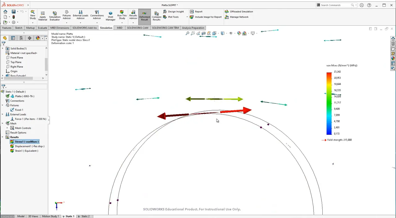
Edit Definition, Advanced Options, Show as tensor plot, draws the principal stresses at each node as arrows (Figure 15.2.12). On a fine mesh this takes a long time to draw, so use a coarser mesh for the picture. Arrows pointing outwards are tension, arrows pointing inwards compression, and the three arrows at a node are perpendicular to each other. At the top of the hole, the large red pair pulls the material apart along the load, and the third principal stress, perpendicular to the plate, is so small that it is visible only at extreme zoom.
A figure for a report needs a plain white background (Apply Scene, Plain White, on the heads-up view toolbar), the fixture and load symbols hidden unless they help, the part zoomed so that the region of interest and the colour bar fill the picture, and a deformation scale that is stated. One plot of the whole part is rarely enough; an Iso Clipping or a section of the critical region shows the reader where the number comes from.
Videos
The examples are worked through on screen, in Swedish, in Plattan (Examples 1 and 2) and SolidWorks Simulation - Plattan revisited (Example 3).