Code
uu = sp.Matrix([1, -2, 3])
vv = sp.Matrix([3, 4, -5])
uv = uu.dot(vv)“The direct product of two vectors \(\mathbf{A}\) and \(\mathbf{B}\) is the scalar quantity obtained by multiplying the product of the magnitudes of the vectors by the cosine of the angle between them.”
— Edwin Bidwell Wilson, Vector Analysis, founded upon the lectures of J. Willard Gibbs, 1901
Two vectors \(\bm u\) and \(\bm v\) that make the angle \(\theta\) with each other have the dot product
\[ \boxed{\bm u\cdot\bm v = |\bm u|\,|\bm v|\cos\theta} \tag{3.6.1}\]
The result is a number, a scalar, which gives the operation its other name, the scalar product. The right-hand side does not care which vector comes first, so \(\bm u\cdot\bm v = \bm v\cdot\bm u\). For any vectors \(\bm u\), \(\bm v\), \(\bm w\) and any real number \(s\) the dot product obeys the rules
\[ \begin{aligned} \bm u\cdot\bm v &= \bm v\cdot\bm u && \text{commutative law} \\ (s\bm u)\cdot\bm v &= s\,(\bm u\cdot\bm v) && \text{associative law for a scalar} \\ (\bm u + \bm v)\cdot\bm w &= \bm u\cdot\bm w + \bm v\cdot\bm w && \text{distributive law} \\ \bm u\cdot\bm 0 &= 0 && \text{zero vector} \end{aligned} \]
so we multiply out brackets of dot products as we would with numbers.
Both lengths in 3.6.1 are positive, so the sign of the dot product is the sign of \(\cos\theta\). It is positive when the vectors make an acute angle, negative when the angle is obtuse and zero when they are perpendicular, Figure 3.6.1.
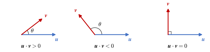
In the video, \(\bm v\) turns away from \(\bm u\) and the dot product is computed from the components of the two arrows. The thick segment on the line of \(\bm u\) is the shadow of \(\bm v\); it shrinks to nothing at the right angle and then falls behind \(\bm u\), where the dot product turns negative.
Two vectors at a right angle are called orthogonal, and the dot product tests for it without any angle:
\[ \bm u\perp\bm v \quad\Longleftrightarrow\quad \bm u\cdot\bm v = 0 \tag{3.6.2}\]
This test is the building block we return to whenever two directions must be perpendicular.
The definition 3.6.1 is used only when the angle is what we seek. When the components are known, we write both vectors in the basis, \(\bm u = u_x\bm i + u_y\bm j + u_z\bm k\) and likewise \(\bm v\), and multiply out the brackets with the rules above. Every term of the result holds the dot product of two basis vectors. These have unit length and are mutually perpendicular, so \(\bm i\cdot\bm i = \bm j\cdot\bm j = \bm k\cdot\bm k = 1\), and the mixed products such as \(\bm i\cdot\bm j\) vanish by 3.6.2. Only the products of matching components survive. On column form we pair the rows of the two vectors, multiply each pair and add the products,
\[ \boxed{\bm u\cdot\bm v = \begin{bmatrix}u_x\\ u_y\\ u_z\end{bmatrix}\cdot\begin{bmatrix}v_x\\ v_y\\ v_z\end{bmatrix} = u_xv_x + u_yv_y + u_zv_z} \tag{3.6.3}\]
The video multiplies out the brackets and then pairs the rows, first in symbols and then with the vectors of Example 1.
In SymPy the dot product of two column vectors is uu.dot(vv); the matrix product uu.T*vv gives the same number inside a \(1\times 1\) matrix.
Grant Sanderson shows in the video below why pairing the rows gives the same number as the shadow picture of 3.6.1. Its second half treats the dot product as a linear map, which we meet again with matrices.
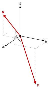
Find the dot product of \(\bm u = [1, -2, 3]^\mathsf{T}\) and \(\bm v = [3, 4, -5]^\mathsf{T}\) in Figure 3.6.2.
The components are known, so 3.6.3 applies directly,
\[ \bm u\cdot\bm v = 1\cdot 3 + (-2)\cdot 4 + 3\cdot(-5) \]
uu = sp.Matrix([1, -2, 3])
vv = sp.Matrix([3, 4, -5])
uv = uu.dot(vv)which gives
\[ \bm u\cdot\bm v = \left[\begin{matrix}1 & -2 & 3\end{matrix}\right]\left[\begin{matrix}3\\4\\-5\end{matrix}\right] = -20 \]
The dot product is negative, so the angle between the vectors is obtuse, as Figure 3.6.2 shows.
Practise the dot product from components below, in the plane or in space. The Python switch turns the exercise into code: the same problem is solved with SymPy and checked when we run it.
The dot product of a vector with itself is the square of its length, since \(\theta = 0\) in 3.6.1. By 3.6.3 that is the Pythagorean length from Chapter 3.5,
\[ |\bm v| = \sqrt{\bm v\cdot\bm v} = \sqrt{v_x^2 + v_y^2 + v_z^2} \tag{3.6.4}\]
and in SymPy vv.norm() and sp.sqrt(vv.dot(vv)) give the same result.
Solving 3.6.1 for the angle gives
\[ \cos\theta = \frac{\bm u\cdot\bm v}{|\bm u|\,|\bm v|}, \qquad 0 \le \theta \le \pi \tag{3.6.5}\]
with all three quantities on the right computed from components. This is the one place where the definition with the angle is used. Elsewhere we avoid angles in a model: they depend on the coordinate system, they hide signs and quadrants, and 3.6.3 and the projection below answer the same questions with components alone.
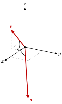
Find the angle between \(\bm u = [3, 2, -4]^\mathsf{T}\) and \(\bm v = [1, -1, 2]^\mathsf{T}\) in Figure 3.6.3.
The three numbers that 3.6.5 needs are
\[ \bm u\cdot\bm v = 3 - 2 - 8 = -7, \qquad |\bm u| = \sqrt{9 + 4 + 16} = \sqrt{29}, \qquad |\bm v| = \sqrt{1 + 1 + 4} = \sqrt 6 \]
so that
\[ \theta = \arccos\frac{-7}{\sqrt{29}\sqrt 6} = \arccos\left(-\frac{7}{\sqrt{174}}\right) \]
uu = sp.Matrix([3, 2, -4])
vv = sp.Matrix([1, -1, 2])
theta = sp.acos(uu.dot(vv)/(uu.norm()*vv.norm()))
In radians and in degrees,
\[ \theta = \operatorname{acos}{\left(- \dfrac{7 \sqrt{174}}{174} \right)} \approx 2.13\text{ rad} \approx 122.1^\circ \]
The angle is obtuse, which the negative dot product told us before any arccos was taken.
Practise the angle between two vectors below. The field accepts expressions such as acos(-7/sqrt(174)), which is evaluated in degrees.
The angles \(\alpha\), \(\beta\) and \(\gamma\) between a vector \(\bm v\) and the \(x\), \(y\) and \(z\) axes, Figure 3.6.4, appear in many textbooks under the name direction cosines. Each is an angle between \(\bm v\) and a basis vector, so 3.6.5 gives them, e.g., \(\cos\alpha = \bm v\cdot\bm i/|\bm v| = v_x/|\bm v|\), and together
\[ \begin{bmatrix}\cos\alpha\\ \cos\beta\\ \cos\gamma\end{bmatrix} = \frac{1}{|\bm v|}\begin{bmatrix}v_x\\ v_y\\ v_z\end{bmatrix} = \bm e_v \]
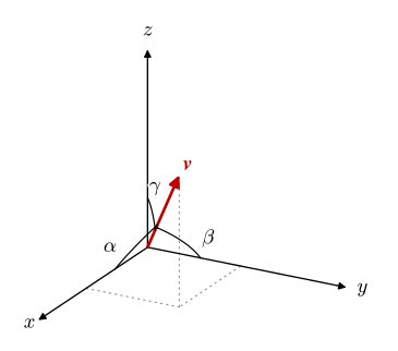
The direction cosines are the components of the unit vector \(\bm e_v\). They hold nothing that \(\bm e_v\) does not, and since \(|\bm e_v| = 1\) they satisfy \(\cos^2\alpha + \cos^2\beta + \cos^2\gamma = 1\). We work with \(\bm e_v\) and compute an angle only when a question asks for one.
The dot product has a picture. The shadow of \(\bm v\) on the line of \(\bm u\) has the signed length \(|\bm v|\cos\theta\), Figure 3.6.5, so 3.6.1 reads
\[ \bm u\cdot\bm v = |\bm u|\,\big(|\bm v|\cos\theta\big) \]
the length of \(\bm u\) times the signed length of the shadow of \(\bm v\). The shadow is a leg of a right triangle with \(\bm v\) as its hypotenuse, and a leg is never longer than the hypotenuse. The absolute value of the dot product therefore never exceeds the product of the lengths,
\[ |\bm u\cdot\bm v| \le |\bm u|\,|\bm v| \tag{3.6.6}\]
the Cauchy–Schwarz inequality, named after Augustin Louis Cauchy (1789–1857) and Hermann Amandus Schwarz (1843–1921).
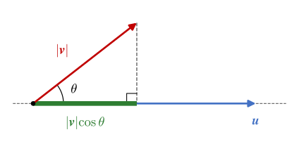
In the video \(\bm v\) turns once around. The outlined rectangle has the sides \(|\bm u|\) and \(|\bm v|\); the filled one has the sides \(|\bm u|\) and the shadow of \(\bm v\), so its area is \(|\bm u\cdot\bm v|\). It fills the outline only when \(\bm v\) lies on the line of \(\bm u\): equality holds only when the vectors are parallel.
The length of a sum follows from 3.6.4 and the rules of the dot product, with 3.6.6 in the third step,
\[ \begin{aligned} |\bm u + \bm v|^2 &= (\bm u + \bm v)\cdot(\bm u + \bm v) = |\bm u|^2 + 2\,\bm u\cdot\bm v + |\bm v|^2 \\ &\le |\bm u|^2 + 2\,|\bm u|\,|\bm v| + |\bm v|^2 = \left(|\bm u| + |\bm v|\right)^2 \end{aligned} \]
Both sides are squares of non-negative numbers, so taking the square root gives the triangle inequality
\[ |\bm u + \bm v| \le |\bm u| + |\bm v| \]
In the triangle of Figure 3.6.6, the side \(\bm u + \bm v\) is never longer than the other two sides together, \(\bm u\) and \(\bm v\) drawn tip to tail.
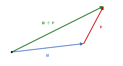
In the video \(\bm v\) turns at the tip of \(\bm u\). The straight path \(|\bm u + \bm v|\) reaches the length of the detour \(|\bm u| + |\bm v|\) only when \(\bm v\) points along \(\bm u\) and the triangle flattens into a line.
The orthogonal projection of a vector \(\bm v\) on another vector \(\bm b\) is the shadow that \(\bm v\) casts on the line of \(\bm b\) when the light falls perpendicular to that line, Figure 3.6.7. The result is a new vector \(\bm p\) on the line of \(\bm b\).
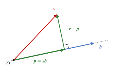
As \(\bm v\) moves, its shadow \(\bm p\) moves along the line of \(\bm b\), and it points against \(\bm b\) when the angle between \(\bm v\) and \(\bm b\) is obtuse.
We read two relations off Figure 3.6.7, and they are all we need to find \(\bm p\):
The first relation leaves one unknown, the number \(s\). Inserting it in the second and multiplying out with the rules of the dot product gives an equation for \(s\),
\[ \begin{aligned} (\bm v - s\bm b)\cdot\bm b &= 0 \\ \bm v\cdot\bm b - s\,\bm b\cdot\bm b &= 0 \\ s &= \frac{\bm v\cdot\bm b}{\bm b\cdot\bm b} \end{aligned} \]
and with \(\bm p = s\bm b\) the projection of \(\bm v\) on \(\bm b\) is
\[ \boxed{\bm p = \operatorname{proj}_{\bm b}\bm v = \frac{\bm v\cdot\bm b}{\bm b\cdot\bm b}\,\bm b} \tag{3.6.7}\]
The video runs the derivation on the drawing. The point \(s\bm b\) slides along \(\bm b\), the dot product \((\bm v - s\bm b)\cdot\bm b\) is computed for each \(s\), and it passes zero exactly where the remainder stands at a right angle to \(\bm b\).
Two kinds of multiplication meet in 3.6.7. The two dot products give numbers, their quotient is the number \(s\), and \(s\) multiplies the vector \(\bm b\). The denominator \(\bm b\cdot\bm b = |\bm b|^2\) removes the length of \(\bm b\), so only its direction matters.
When \(\bm b\) is a unit vector \(\bm e\), the denominator is \(\bm e\cdot\bm e = 1\) and the division disappears. One dot product gives the number and the number scales \(\bm e\),
\[ \bm p = (\bm v\cdot\bm e)\,\bm e, \qquad |\bm e| = 1 \tag{3.6.8}\]
the cheap projection. It pays to keep a direction as a unit vector. The basis vectors are the simplest case: the cheap projection of \(\bm v\) on \(\bm i\) is \((\bm v\cdot\bm i)\,\bm i = v_x\bm i\), the composant of \(\bm v\) along \(x\). Any other direction \(\bm b\) is normalised once, \(\bm e_b = \bm b/|\bm b|\), and every projection on it is then cheap.
The number \(\bm v\cdot\bm e_b\) is the signed length of the shadow, the component of \(\bm v\) along \(\bm b\). It is negative when \(\bm p\) points against \(\bm b\). Swapping the roles changes the result, \(\operatorname{proj}_{\bm b}\bm v \ne \operatorname{proj}_{\bm v}\bm b\), except when the vectors are orthogonal and both projections are \(\bm 0\).
The two relations of the derivation reach far beyond this formula. The distance from a point to a line, the mirror image of a point and the shortest distance between two lines in Chapter 3.8 are all found the same way: write what is parallel as a multiple, write what is perpendicular as a zero dot product, and solve.
In SymPy we write the projection as it stands in 3.6.7, and v.project(b) is the built-in equivalent.
def proj(v, b):
    # two dot products give the number s, which then scales b
    return v.dot(b)/b.dot(b)*b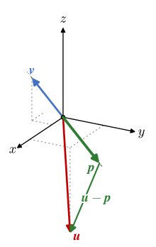
Find the projection of \(\bm u = [3, 2, -4]^\mathsf{T}\) on \(\bm v = [1, -1, 2]^\mathsf{T}\), Figure 3.6.8, and compare it with the projection of \(\bm v\) on \(\bm u\).
With \(\bm u\cdot\bm v = -7\) from Example 2, \(\bm v\cdot\bm v = 6\) and \(\bm u\cdot\bm u = 29\), 3.6.7 gives
\[ \operatorname{proj}_{\bm v}\bm u = \frac{\bm u\cdot\bm v}{\bm v\cdot\bm v}\,\bm v = -\frac{7}{6}\begin{bmatrix}1\\-1\\2\end{bmatrix}, \qquad \operatorname{proj}_{\bm u}\bm v = \frac{\bm v\cdot\bm u}{\bm u\cdot\bm u}\,\bm u = -\frac{7}{29}\begin{bmatrix}3\\2\\-4\end{bmatrix} \]
and the remainder of the first must be perpendicular to \(\bm v\), \((\bm u - \operatorname{proj}_{\bm v}\bm u)\cdot\bm v = 0\).
uu = sp.Matrix([3, 2, -4])
vv = sp.Matrix([1, -1, 2])
pp_u_on_v = proj(uu, vv)
pp_v_on_u = proj(vv, uu)
check = (uu - pp_u_on_v).dot(vv)
The two projections and the check are
\[ \begin{aligned}\operatorname{proj}_{\bm v}\bm u &= \left[\begin{matrix}- \dfrac{7}{6} & \dfrac{7}{6} & - \dfrac{7}{3}\end{matrix}\right]^\mathsf{T}\\ \operatorname{proj}_{\bm u}\bm v &= \left[\begin{matrix}- \dfrac{21}{29} & - \dfrac{14}{29} & \dfrac{28}{29}\end{matrix}\right]^\mathsf{T}\\ (\bm u - \operatorname{proj}_{\bm v}\bm u)\cdot\bm v &= 0\end{aligned} \]
The two projections differ in length and direction. Both carry the factor \(-7\), the negative dot product, so each points against the vector it lies on.
Practise the projection below. Fractions such as -7/6 may be typed as they are; once the answer is right, the projection and the remainder are drawn.
Find a unit vector in the direction of the projection of \(\bm v = [1, -1, 2]^\mathsf{T}\) on \(\bm u = [3, 2, -4]^\mathsf{T}\), the vectors of Figure 3.6.3.
The order of the operations matters: project first, then normalise,
\[ \bm p = \operatorname{proj}_{\bm u}\bm v, \qquad \bm e_p = \frac{\bm p}{|\bm p|} \]
Normalising \(\bm v\) first and projecting the unit vector gives a vector of length \(|\cos\theta| < 1\), no unit vector.
pp = proj(vv, uu)
ee_p = pp/pp.norm()
The unit vector is
\[ \bm e_p = \left[\begin{matrix}- \dfrac{3 \sqrt{29}}{29} & - \dfrac{2 \sqrt{29}}{29} & \dfrac{4 \sqrt{29}}{29}\end{matrix}\right]^\mathsf{T} = \left[\begin{matrix}-3 & -2 & 4\end{matrix}\right]^\mathsf{T}/\sqrt{29} \]
It is \(-\bm u/|\bm u|\). The projection lies on the line of \(\bm u\) and points against \(\bm u\), so its unit vector is the unit vector of \(\bm u\) reversed.
Practise the order of the operations below: project first, then normalise.
The projection splits any vector into two perpendicular parts,
\[ \bm v = \underbrace{\operatorname{proj}_{\bm b}\bm v}_{\parallel\,\bm b} + \underbrace{(\bm v - \operatorname{proj}_{\bm b}\bm v)}_{\perp\,\bm b} \tag{3.6.9}\]
The first part lies along the direction of \(\bm b\) and the second across it. The length of the second part is the distance from the tip of \(\bm v\) to the line through the origin along \(\bm b\).
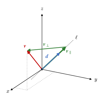
The line \(\ell\) in Figure 3.6.9 passes through the origin in the direction \(\bm d = [1, 2, 2]^\mathsf{T}\). Split \(\bm v = [4, 1, 3]^\mathsf{T}\) into a part along \(\ell\) and a part perpendicular to \(\ell\).
With \(\bm v\cdot\bm d = 4 + 2 + 6 = 12\) and \(\bm d\cdot\bm d = 9\) the procedure gives
\[ \begin{aligned} \bm v_\parallel &= \frac{\bm v\cdot\bm d}{\bm d\cdot\bm d}\,\bm d = \frac{4}{3}\begin{bmatrix}1\\2\\2\end{bmatrix} \\ \bm v_\perp &= \bm v - \bm v_\parallel \end{aligned} \]
with the checks \(\bm v_\perp\cdot\bm d = 0\) and \(\bm v_\parallel + \bm v_\perp = \bm v\).
vv = sp.Matrix([4, 1, 3])
dd = sp.Matrix([1, 2, 2])
vv_par = proj(vv, dd)
vv_perp = vv - vv_par
checks = [vv_perp.dot(dd), vv_par + vv_perp - vv]
The two parts are
\[ \begin{aligned}\bm v_\parallel &= \left[\begin{matrix}\dfrac{4}{3} & \dfrac{8}{3} & \dfrac{8}{3}\end{matrix}\right]^\mathsf{T}\\ \bm v_\perp &= \left[\begin{matrix}\dfrac{8}{3} & - \dfrac{5}{3} & \dfrac{1}{3}\end{matrix}\right]^\mathsf{T}\end{aligned} \]
and both checks hold,
\[ \bm v_\perp\cdot\bm d = 0, \qquad \bm v_\parallel + \bm v_\perp - \bm v = \left[\begin{matrix}0 & 0 & 0\end{matrix}\right]^\mathsf{T} \]
The length \(|\bm v_\perp| = \sqrt{(64 + 25 + 1)/9} = \sqrt{10} \approx 3.16\) is the distance from the point \((4, 1, 3)\) to the line \(\ell\).
Practise the split along a line in space below.
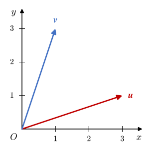
Split \(\bm u = [3, 1]^\mathsf{T}\) in Figure 3.6.10 into a part parallel to \(\bm v = [1, 3]^\mathsf{T}\) and a part perpendicular to it.
Here \(\bm u\cdot\bm v = 3 + 3 = 6\) and \(\bm v\cdot\bm v = 10\), so
\[ \begin{aligned} \bm u_\parallel &= \frac{6}{10}\begin{bmatrix}1\\3\end{bmatrix} \\ \bm u_\perp &= \bm u - \bm u_\parallel \end{aligned} \]
and the check \(\bm u_\parallel\cdot\bm u_\perp = 0\) confirms that the parts are perpendicular.
uu = sp.Matrix([3, 1])
vv = sp.Matrix([1, 3])
uu_par = proj(uu, vv)
uu_perp = uu - uu_par
check = uu_par.dot(uu_perp)
The parts and the check are
\[ \begin{aligned}\bm u_\parallel &= \left[\begin{matrix}\dfrac{3}{5} & \dfrac{9}{5}\end{matrix}\right]^\mathsf{T}, \quad |\bm u_\parallel| = \dfrac{3 \sqrt{10}}{5}\\ \bm u_\perp &= \left[\begin{matrix}\dfrac{12}{5} & - \dfrac{4}{5}\end{matrix}\right]^\mathsf{T}, \quad |\bm u_\perp| = \dfrac{4 \sqrt{10}}{5}\\ \bm u_\parallel\cdot\bm u_\perp &= 0\end{aligned} \]
Figure 3.6.11 draws the two parts from the computed components, tip to tail.
def arrow(ax, p0, w, color, label):
    ax.annotate('', xy=(p0[0] + w[0], p0[1] + w[1]), xytext=(p0[0], p0[1]),
                arrowprops=dict(arrowstyle='-|>', color=color, lw=2, shrinkA=0, shrinkB=0))
    ax.text(p0[0] + 0.55*w[0], p0[1] + 0.55*w[1], label, color=color, fontsize=13,
            ha='right', va='bottom')

u, v = np.array(uu, float).ravel(), np.array(vv, float).ravel()
u_par, u_perp = np.array(uu_par, float).ravel(), np.array(uu_perp, float).ravel()

fig, ax = plt.subplots(figsize=(4.5, 4.5))
arrow(ax, (0, 0), v, '#4472c4', r'$\boldsymbol{v}$')
arrow(ax, (0, 0), u, '#c00000', r'$\boldsymbol{u}$')
arrow(ax, (0, 0), u_par, '#2e7d32', r'$\boldsymbol{u}_\parallel$')
# drawn from the tip of the parallel part, the perpendicular part must end at the tip of u
arrow(ax, u_par, u_perp, '#2e7d32', r'$\boldsymbol{u}_\perp$')
ax.set_aspect('equal')
ax.set_xlim(0, 3)
ax.set_ylim(0, 3)
ax.set_xticks([0, 1, 2, 3])
ax.set_yticks([0, 1, 2, 3])
ax.set_xlabel('$x$')
ax.set_ylabel('$y$')
ax.grid(True, alpha=0.4)
plt.show()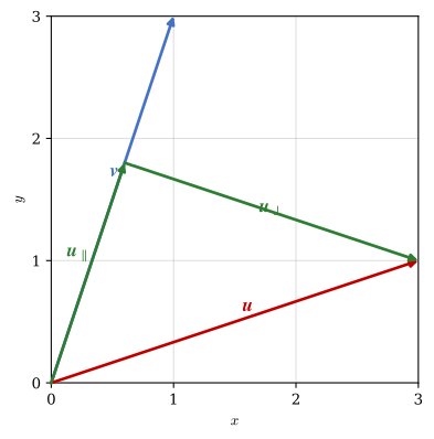
The video builds the same split: the drop from the tip of \(\bm u\) to the line of \(\bm v\), the two parts, and the perpendicular part moved to the origin, where the two parts span a rectangle with \(\bm u\) as its diagonal.
Practise the split in the plane below. The two parts are drawn tip to tail once they are right.
A vector of the form
\[ \bm v = \lambda_1\bm a_1 + \lambda_2\bm a_2 + \dots + \lambda_n\bm a_n \]
with numbers \(\lambda_1, \dots, \lambda_n\) is a linear combination of the vectors \(\bm a_1, \dots, \bm a_n\). The vectors are linearly dependent when one of them is a linear combination of the others, or equivalently, when there are numbers \(\lambda_1, \dots, \lambda_n\), not all zero, such that \(\lambda_1\bm a_1 + \dots + \lambda_n\bm a_n = \bm 0\). Otherwise they are linearly independent, and that sum is zero only when every \(\lambda_k = 0\).
Two vectors are dependent when they are parallel, which is equality in 3.6.6, \(|\bm a\cdot\bm b| = |\bm a|\,|\bm b|\). Three vectors in space are dependent when they lie in one plane. For \(\bm a_1 = [1, 2, 3]^\mathsf{T}\), \(\bm a_2 = [2, -1, 0]^\mathsf{T}\) and \(\bm a_3 = [4, 3, 6]^\mathsf{T}\) the equation \(\lambda_1\bm a_1 + \lambda_2\bm a_2 + \lambda_3\bm a_3 = \bm 0\) is a linear system for the \(\lambda_k\), whose non-zero solutions SymPy finds as the null space of the matrix with the vectors as columns.
A = sp.Matrix.hstack(sp.Matrix([1, 2, 3]), sp.Matrix([2, -1, 0]), sp.Matrix([4, 3, 6]))
lambdas = A.nullspace()       # empty for independent vectors
The null space is spanned by
\[ \begin{bmatrix}\lambda_1\\ \lambda_2\\ \lambda_3\end{bmatrix} = \left[\begin{matrix}-2\\-1\\1\end{matrix}\right] \]
so \(\bm a_3 = 2\bm a_1 + \bm a_2\) and the three vectors are dependent. Three independent vectors can serve as a basis for a coordinate system. The basis \(\bm i\), \(\bm j\), \(\bm k\) is the special case that is both orthogonal and normalised; a basis that is neither is called oblique.