When every component of a vector is a function of the same real variable \(t\), the vector is a vector-valued function of \(t\),
\[
\bm r(t) = [x(t),\ y(t),\ z(t)]^\mathsf{T}
\]
The components \(x(t)\), \(y(t)\) and \(z(t)\) are the coordinate functions. As \(t\) runs through an interval, the tip of \(\bm r(t)\) traces a curve, and we call \(\bm r(t)\) a parameter curve with the parameter\(t\). Differentiation and integration work one coordinate function at a time,
so a vector-valued function asks for nothing beyond the calculus of one variable, done three times. These rules are applied to motion in particle kinematics.
The tangent vector as the limit of a chord
Two values of the parameter, \(t\) and \(t + \Delta t\), give two points on the curve. The vector from the first to the second is the chord
Dividing by the number \(\Delta t\) changes the length of the chord and leaves its direction alone. As \(\Delta t\) shrinks, the second point slides toward the first, the chord turns toward the direction in which the curve leaves \(\bm r(t)\), and the quotient settles on a finite vector,
the tangent vector of the curve at \(\bm r(t)\), Figure 3.9.1. The dot over \(\bm r\) denotes the derivative with respect to \(t\), and two dots, \(\ddot{\bm r}\), the second derivative.
Figure 3.9.1: The chord \(\Delta\bm r\) (red) from \(\bm r(t)\) to \(\bm r(t+\Delta t)\), and the quotient \(\Delta\bm r/\Delta t\) (green) drawn from \(\bm r(t)\). As \(\Delta t\) shrinks the quotient turns onto the tangent line and stops changing: it has become \(\dot{\bm r}(t)\).
Divided by its own length, the tangent vector gives the unit tangent \(\bm e_t = \dot{\bm r}/|\dot{\bm r}|\), the direction of the curve at \(\bm r(t)\).
Arc length
Over a short step \(dt\) the tip of \(\bm r\) moves by \(d\bm r = \dot{\bm r}\,dt\), a chord so short that it lies on the curve. Its length is the length of a vector, which the dot product gives as \(|\bm a| = \sqrt{\bm a \cdot \bm a}\), so the small piece of the curve has the length
\[
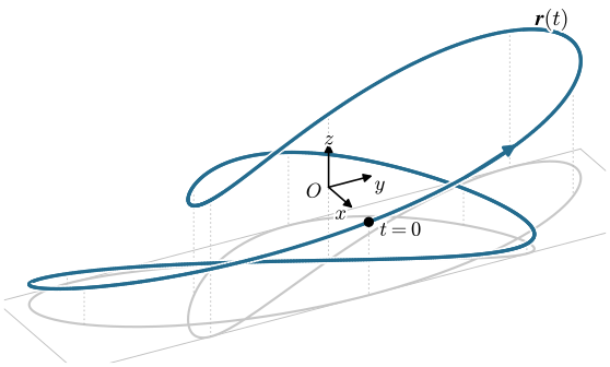
\bm r(t) = 5\,[\cos 3t,\ (\cos t + 3)\sin 2t,\ \sin t]^\mathsf{T}, \qquad t \in [0, 2\pi]
\]
Determine (a) the arc length of the curve, (b) the tangent vector \(\dot{\bm r}(t)\) and the largest and smallest value of its length \(|\dot{\bm r}(t)|\), and (c) the second derivative \(\ddot{\bm r}(t)\) and the largest and smallest value of \(|\ddot{\bm r}(t)|\).
Figure 3.9.2: The closed curve \(\bm r(t)\), with its start at \(t = 0\) and the direction of increasing \(t\). The grey curve is its projection on the plane \(z = -5\), and the dotted lines join the two.
Everything follows from \(\bm r(t)\) and its first two derivatives,
The extremes of \(|\dot{\bm r}(t)|\) lie where its derivative with respect to \(t\) is zero. The second half of the interval repeats the first in reverse: \(\bm r(2\pi - t)\) is \(\bm r(t)\) with \(y\) and \(z\) negated, the curve turned half a revolution about the \(x\) axis, so \(|\dot{\bm r}(2\pi - t)| = |\dot{\bm r}(t)|\) and \(|\ddot{\bm r}(2\pi - t)| = |\ddot{\bm r}(t)|\). We therefore sample \(|\dot{\bm r}(t)|\) over \(t \in [0, \pi]\), refine the largest and the smallest sample with a local search, and treat \(|\ddot{\bm r}(t)|\) the same way.
Code
t = sp.symbols('t', real=True)rr =5*sp.Matrix([sp.cos(3*t), (sp.cos(t) +3)*sp.sin(2*t), sp.sin(t)])rr_dot = rr.diff(t) # differentiated entry by entry: the tangent vectorrr_ddot = rr_dot.diff(t) # and once morelen_dot = sp.sqrt(rr_dot.dot(rr_dot)) # |r'| through the dot productlen_ddot = sp.sqrt(rr_ddot.dot(rr_ddot))
Differentiating the curve entry by entry gives the tangent vector
\[ \dot{\bm r}(t) =\left[\begin{matrix}- 15 \sin{\left(3 t \right)}\\10 \left(\cos{\left(t \right)} + 3\right) \cos{\left(2 t \right)} - 5 \sin{\left(t \right)} \sin{\left(2 t \right)}\\5 \cos{\left(t \right)}\end{matrix}\right] \]
and once more the second derivative
\[ \ddot{\bm r}(t) =\left[\begin{matrix}- 45 \cos{\left(3 t \right)}\\- 20 \left(\cos{\left(t \right)} + 3\right) \sin{\left(2 t \right)} - 20 \sin{\left(t \right)} \cos{\left(2 t \right)} - 5 \sin{\left(2 t \right)} \cos{\left(t \right)}\\- 5 \sin{\left(t \right)}\end{matrix}\right] \]
Code
len_dot_f = sp.lambdify(t, len_dot, 'numpy')len_ddot_f = sp.lambdify(t, len_ddot, 'numpy')# |r'| has no antiderivative in closed form; quad integrates it adaptivelyL, L_err = quad(len_dot_f, 0, 2*np.pi, limit=200)def extremes(f, T=np.linspace(0, np.pi, 2001)):"""Largest and smallest value of f over the first half of the interval: the best sample, then a local search around it, so an extreme between two samples is not missed.""" out = {}for name, sign in (('max', -1), ('min', 1)): k = np.argmin(sign*f(T)) lo, hi = T[max(k -1, 0)], T[min(k +1, len(T) -1)] res = minimize_scalar(lambda s: sign*f(s), bounds=(lo, hi), method='bounded', options={'xatol': 1e-10}) out[name] = (res.x, f(res.x))return outd_ext = extremes(len_dot_f)dd_ext = extremes(len_ddot_f)
For (a), the numerical integral of \(|\dot{\bm r}|\) over the interval gives the arc length,
\[ L = \int_0^{2\pi} |\dot{\bm r}|\,dt =143.96 \]
A check that leans on nothing but the definition of length: replace the curve by \(N\) chords between the points \(\bm r(t_i)\), \(t_i = 2\pi i/N\), and add their lengths, \(L_N = \sum_i |\bm r(t_{i+1}) - \bm r(t_i)|\). Every chord is shorter than the arc it cuts off, so \(L_N\) grows toward \(L\) from below as \(N\) grows.
Code
r_f = sp.lambdify(t, rr, 'numpy')def chord_length(N): pts = np.array([np.ravel(r_f(ti)) for ti in np.linspace(0, 2*np.pi, N +1)])return np.sum(np.linalg.norm(np.diff(pts, axis=0), axis=1))L_N = {N: chord_length(N) for N in (10, 100, 1000)}
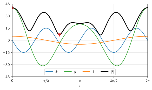
Figure 3.9.3: The components of the tangent vector (thin) and its length \(|\dot{\bm r}|\) (black). The red triangles mark the largest and the smallest length.
The largest and smallest length of the tangent vector, and where they occur, are
\[ \begin{aligned}|\dot{\bm r}|_{\max} &=40.31\quad \text{at } t =0\\ |\dot{\bm r}|_{\min} &=6.54\quad \text{at } t =2.19\end{aligned} \]
The tangent vector is longest at the start, where \(\dot{\bm r}(0) = [0,\ 40,\ 5]^\mathsf{T}\) points almost straight along \(y\). By the symmetry of the curve the smallest length occurs a second time at \(t = 2\pi - 2.19 = 4.09\), as Figure 3.9.3 shows. In Figure 3.9.4 the point \(\bm r(t)\) runs once round the curve with \(\dot{\bm r}(t)\) drawn at it.
Figure 3.9.4: The point \(\bm r(t)\) (yellow) for \(t\) from \(0\) to \(2\pi\). The red arrow is the tangent vector \(\dot{\bm r}(t)\), scaled down, and the number on the right its length. The curve is drawn brighter where it is nearer the viewer.
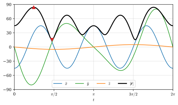
For (c), Figure 3.9.5 shows the length of the second derivative with its components.
Figure 3.9.5: The components of the second derivative (thin) and its length \(|\ddot{\bm r}|\) (black). The red triangles mark the largest and the smallest length.
The largest and the smallest length of the second derivative are
\[ \begin{aligned}|\ddot{\bm r}|_{\max} &=84.08\quad \text{at } t =0.767\\ |\ddot{\bm r}|_{\min} &=15.33\quad \text{at } t =1.493\end{aligned} \]
Each extreme occurs again at \(2\pi - t\). The arc length belongs to the curve and the derivatives to the parameter: tracing the same curve as \(\bm r(t/2)\), \(t \in [0, 4\pi]\), leaves \(L\) unchanged, while by the chain rule the tangent vector is halved and the second derivative drops to a quarter.
Line integrals
A vector field\(\bm F\) attaches a vector to every point, \(\bm F(x, y) = [F_x(x, y),\ F_y(x, y)]^\mathsf{T}\) in the plane. Along a curve we can ask how much of the field points along the curve, added up over its whole length. On one short piece \(d\bm r\) of the curve the field is constant and the piece is straight, and the dot product\(\bm F \cdot d\bm r\) keeps only the component of \(\bm F\) along the piece. Adding the pieces gives the line integral of \(\bm F\) along the curve \(C\), Figure 3.9.7,
\[
\int_C \bm F \cdot d\bm r = \int_{s_a}^{s_b} \bm F(\bm r(s)) \cdot \frac{d\bm r}{ds}\,ds
\]
where \(\bm r(s) = [x(s),\ y(s),\ z(s)]^\mathsf{T}\) is the curve with the parameter \(s\). A component of \(\bm F\) perpendicular to the curve drops out of the dot product and adds nothing. A plane curve given as \(y = y(x)\) uses \(x\) itself as the parameter, \(\bm r(x) = [x,\ y(x)]^\mathsf{T}\) and \(d\bm r/dx = [1,\ y'(x)]^\mathsf{T}\).
Example 2: A line integral along a cosine curve
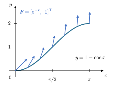
Evaluate the line integral of the vector field \(\bm F(x, y) = [\mathrm{e}^{-x},\ 1]^\mathsf{T}\) along the curve \(C\): \(y = 1 - \cos x\), \(x \in [0, \pi]\), Figure 3.9.6.
Figure 3.9.6: The curve \(y = 1 - \cos x\) and the field \(\bm F = [\mathrm{e}^{-x},\ 1]^\mathsf{T}\) at seven of its points. The field leans along \(x\) near \(x = 0\) and is almost parallel to \(y\) at \(x = \pi\).
Both the field and the direction of the curve change with \(x\), so \(x\) is the parameter. The curve and its derivative are
x = sp.symbols('x', real=True)FF = sp.Matrix([sp.exp(-x), 1]) # the field, evaluated on the curverr_x = sp.Matrix([x, 1- sp.cos(x)]) # the curve with x as parameterintegrand = FF.dot(rr_x.diff(x)) # F . dr/dxI = sp.integrate(integrand, (x, 0, sp.pi))
SymPy integrates \(\bm F \cdot d\bm r/dx\) to the same result,
\[ I =3 - e^{- \pi}=2.957 \]
The integral is the limit of the sum it was built from. Splitting the curve into \(N\) chords \(\Delta\bm r_i = \bm r(x_{i+1}) - \bm r(x_i)\) and taking the field at the start of each chord gives
The sums approach \(3 - \mathrm{e}^{-\pi} = 2.957\) from above, because \(\mathrm{e}^{-x}\) falls along each chord and its value at the start of the chord is the largest on it.
Figure 3.9.7: The line integral as a sum. Each chord \(\Delta\bm r_i\) (green) adds \(\bm F_i \cdot \Delta\bm r_i\) to the bar on the right, with \(\bm F_i\) (red) the field at its start. With more and shorter chords the sum settles on the integral \(3 - \mathrm{e}^{-\pi}\).
The two terms of the integrand split the result. The component \(F_y = 1\) is constant and contributes \(\int_0^\pi \sin x\,dx = 2\), the rise of the curve from \(y = 0\) to \(y = 2\), whatever its shape between the end points. The component \(F_x = \mathrm{e}^{-x}\) contributes \(\int_0^\pi \mathrm{e}^{-x}\,dx = 1 - \mathrm{e}^{-\pi}\), and since it depends on \(x\) alone, here too the shape of the curve plays no part. A field whose \(x\) component depended on \(y\) would in general give different values along different curves between the same end points.
Modelling with vectors
Problems modelled with vectors come down to a small set of techniques. Most of them are two relations,
\[
\bm a \parallel \bm b \;\Rightarrow\; \bm a = s\bm b, \qquad\qquad
\bm a \perp \bm b \;\Rightarrow\; \bm a \cdot \bm b = 0
\]
and the rest of the toolbox is in the table.
Relation
Use
\(\bm a \pm \bm b = [a_x \pm b_x,\ a_y \pm b_y,\ a_z \pm b_z]^\mathsf{T}\)