When we tighten a nut, its thread pulls the bolt through it. The bolt stretches, and the plates between the head and the nut are squeezed together. The tensile force this builds up in the bolt is the preload\(F_0\). It keeps the joint closed under load, it keeps most of a fluctuating load away from the bolt, and through friction between the plates it carries shear loads without the bolt touching the hole. A common target is a preload that stresses the bolt to about 70 % of its yield strength.
We cannot measure the preload with a wrench, only the moment we apply to the nut. The first half of this chapter derives the relation between the two, from the friction in the thread and under the head, and arrives at the formula found in Karl Björk’s tables [1] and in the bolted joint configurator at the end of the chapter. The second half follows the preloaded joint under an external load, with the joint diagram and the pressure cone that gives the stiffness of the clamped plates.
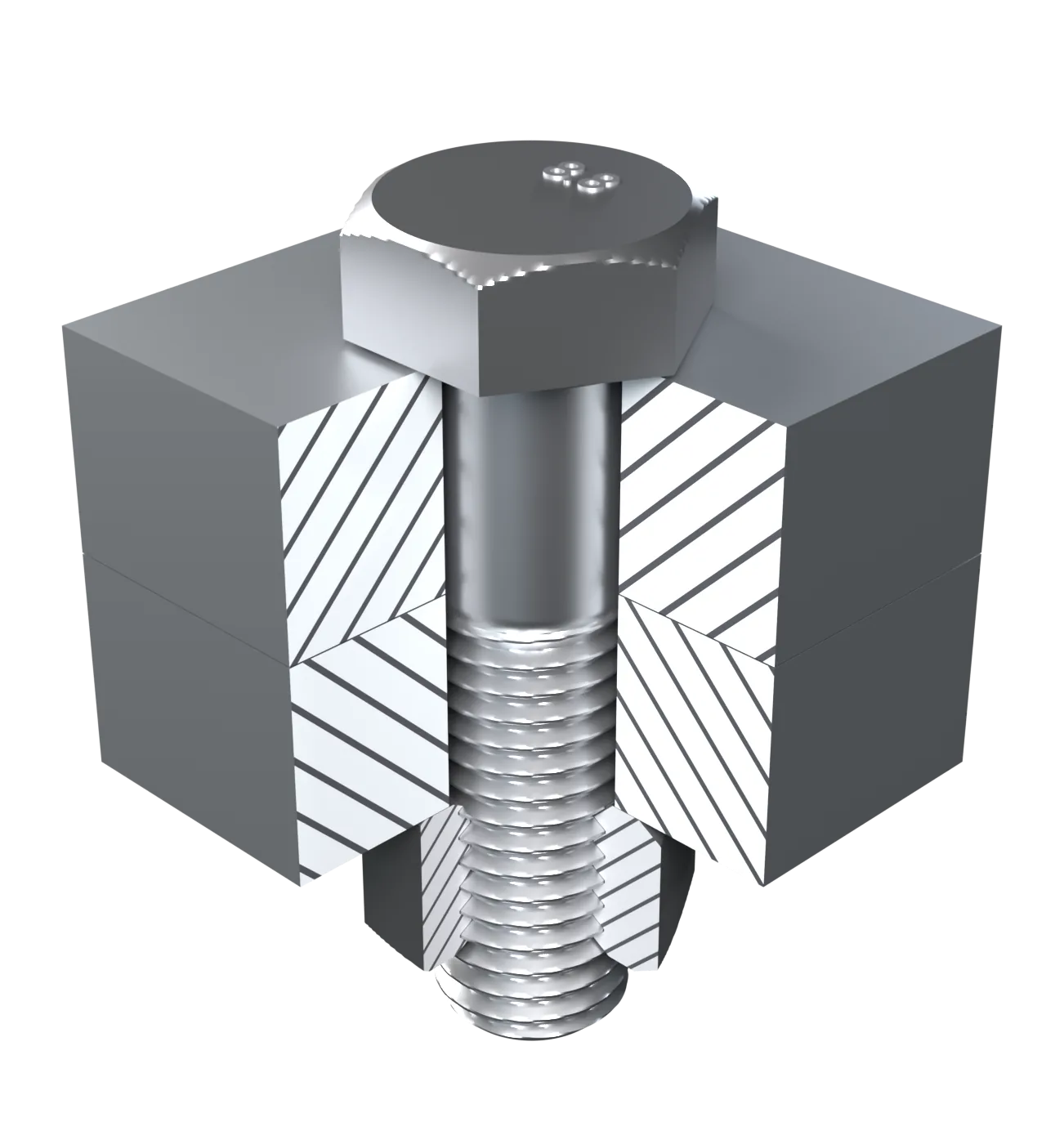
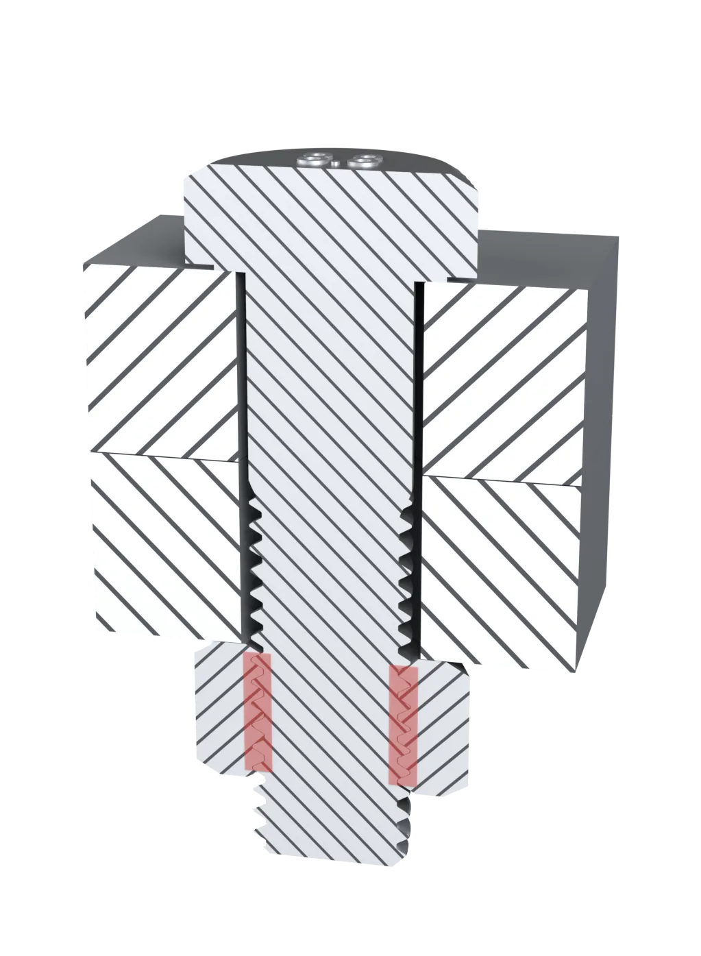
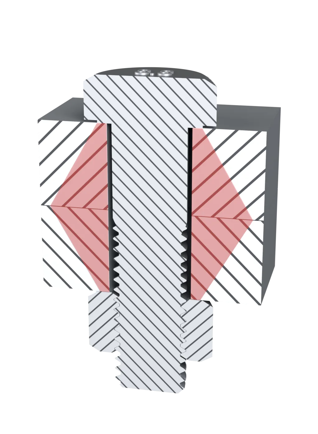
Figure 9.6.1: An M12 bolt clamping two plates, with a quarter of the plates and the nut cut away.
Figure 9.6.2: The Incredible Strength of Bolted Joints, by The Efficient Engineer: preload, tension and shear joints, and the ways the preload is controlled.
The metric thread
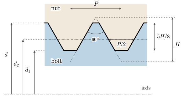
The metric thread of ISO 68-1 has straight flanks at \(60^\circ\) to each other, so each flank makes the angle \(\alpha = 30^\circ\) with the plane normal to the axis (Figure 9.6.3). The pitch\(P\) is the distance between neighbouring threads. The pitch diameter\(d_2\) lies where the thread and the gap between threads are equally wide, \(P/2\) each, and it is the diameter on which the thread forces act in what follows. For the single-start threads of ordinary bolts one turn advances the nut by \(P\).
Figure 9.6.3: The ISO 68-1 basic profile. The bolt and the nut share the same profile line, with the major diameter \(d\), the pitch diameter \(d_2\) and the minor diameter \(d_1\) measured from the axis.
The bolt does not break at the minor diameter but in a somewhat larger section, so strength calculations use the tensile stress area\(A_s = \frac{\pi}{4}\left(\frac{d_2 + d_3}{2}\right)^2\), where \(d_3 = d_1 - H/6\) is the root diameter of the bolt and \(H = \frac{\sqrt 3}{2}P\). For M12, with \(P = 1.75\) mm and \(d_2 = 10.863\) mm, it is \(A_s = 84.3\) mm².
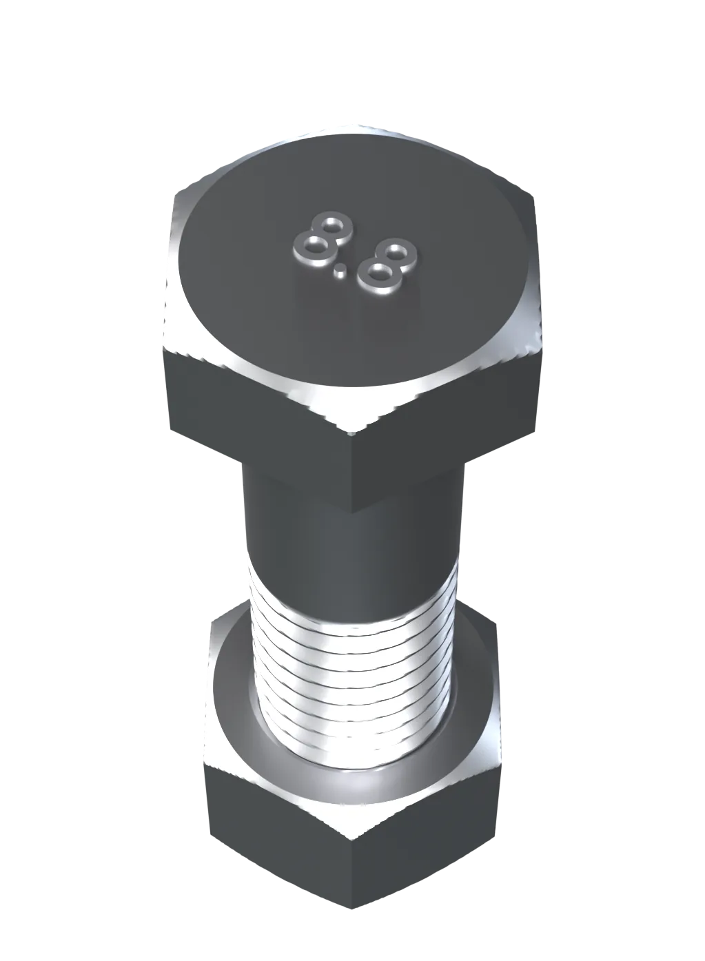
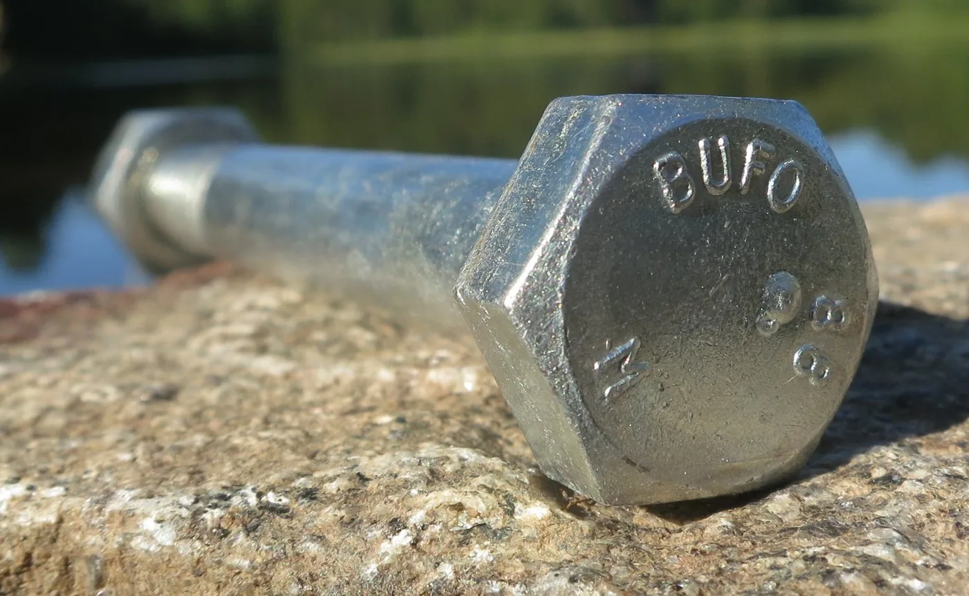
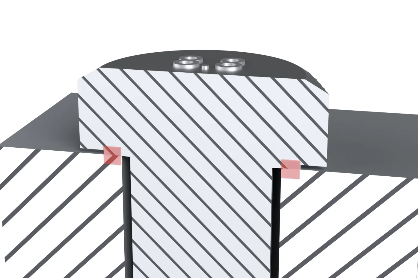
The head of a steel bolt carries its property class, for instance 8.8 (Figure 9.6.4). The first number is a hundredth of the tensile strength, \(R_m = 800\) MPa, and the second is ten times the ratio of yield to tensile strength, so \(R_{p0.2} = 0.8 \cdot 800 = 640\) MPa. Classes 10.9 and 12.9 are stronger on the same pattern.
(a) A render of the M12 bolt with its nut.
(b) An M12 bolt by Bulten, Hallstahammar, marked BUFO and 8.8.
Figure 9.6.4: The property class is stamped on the head.
The tightening torque
The moment \(M_t\) on the wrench has three jobs: it stretches the bolt, it overcomes the friction in the thread, and it overcomes the friction under the head or nut. The first two are the screw of the friction chapter, with a different thread profile; the third is new. We follow the derivation Budynas and Nisbett give for power screws and bolts [2].
(a) Thread contact
(b) Contact under the head
Figure 9.6.5: The two surfaces that slide while the bolt is tightened, marked red in a section through the joint.
The thread as an incline
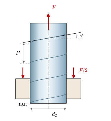
The bolt carries the axial force \(F\), and the nut is held by the clamped plates (Figure 9.6.6). One turn of the thread on the pitch cylinder rises by \(P\) over the circumference \(\pi d_2\). Unrolled, it is an incline (Figure 9.6.7) at the lead angle
\[
\tan\varphi = \frac{P}{\pi d_2}
\tag{9.6.1}\]
Figure 9.6.6: A portion of the bolt with its thread on the pitch cylinder of diameter \(d_2\). The bolt carries \(F\); the clamped plates press on the nut.
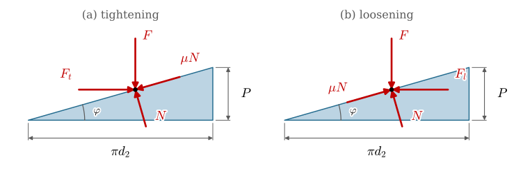
A small piece of the nut thread then rests on the incline. When we tighten, the circumferential force \(F_t\) pushes it up the incline and the friction \(\mu N\) acts down it; when we loosen, \(F_l\) pushes it down and the friction reverses.
Figure 9.6.7: One turn of the thread unrolled into an incline of base \(\pi d_2\) and height \(P\), with the forces on a piece of the nut thread.
Equilibrium of the piece in Figure 9.6.7 (a), along and normal to the axis, gives
the results 5.6.2 and 5.6.3 of the friction chapter. When \(\rho >
\varphi\) the loosening moment is positive: the bolt is self-locking and holds its preload without help.
The flank angle
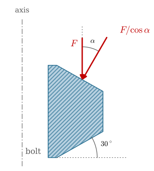
A square thread carries the axial force on a flank normal to the axis. The metric flank is inclined by \(\alpha = 30^\circ\) (Figure 9.6.8), so to carry the axial force \(F\) the flank must push back with the normal force \(F/\cos\alpha\), and the friction grows to \(\mu_g F/\cos\alpha\). The flank wedges the nut onto the bolt. Neglecting the small lead angle in this tilt [2], the thread acts as a square thread with the friction coefficient \(\mu_g/\cos\alpha\), so the friction angle of the thread is
The subscript \(g\) marks the thread (Swedish gänga), as in Björk.
Figure 9.6.8: A bolt thread in an axial section. The axial force \(F\) on the flank requires the normal force \(F/\cos\alpha\).
Friction under the head
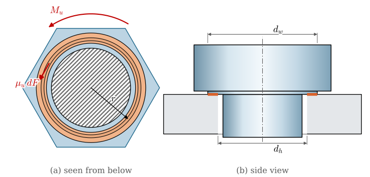
The head, or the nut, turns on its bearing surface, the ring between the hole diameter \(d_h\) and the outer diameter \(d_w\) of the bearing face (Figure 9.6.9). The preload presses this ring with the pressure \(p = F/\big(\pi(r_w^2 - r_h^2)\big)\), which we take as uniform, with \(r_w = d_w/2\) and \(r_h = d_h/2\). We slice the ring into onion rings, as the clutch of the friction chapter. The ring at radius \(r\) of width \(dr\) carries \(dF = p\,2\pi r\,dr\), and its friction \(\mu_u\,dF\) acts at the lever arm \(r\), so
The bearing ring is narrow, so its mean radius \(r_m\) is close to the exact lever arm: for M12 with \(d_w = 16.6\) mm and \(d_h = 13.5\) mm the two are 7.53 and 7.55 mm.
Figure 9.6.9: Friction under the head. (a) The bearing ring seen from below, with one onion ring of radius \(r\). (b) The ring lies between the hole diameter \(d_h\) and the bearing face diameter \(d_w\).
Tightening and loosening torque
Adding 9.6.3 and 9.6.5 for the preload \(F = F_0\) gives the moment needed to tighten the bolt and the moment needed to loosen it,
with \(\tan\varphi = P/(\pi d_2)\) and \(\tan\rho = \mu_g/\cos 30^\circ\). These are the expressions in Björk [1] and in the configurator below. Budynas and Nisbett write the same result as \(M_t = K F_0 d\), with the torque coefficient\(K = \frac{d_2}{2d}\tan(\varphi + \rho) + \frac{\mu_u r_m}{d}\), and note that \(K \approx 0.2\) for unlubricated steel bolts of any size [2].
Example 1: Tightening an M12 bolt
The joint of Figure 9.6.1 has an M12 bolt of class 8.8, to be tightened to a preload of 70 % of its yield force, \(F_0 = 0.7\,R_{p0.2}A_s\). The bearing face has \(d_w = 16.6\) mm, the hole \(d_h = 13.5\) mm, and both friction coefficients are \(\mu_g = \mu_u = 0.15\). Find the tightening and loosening torque, the torque coefficient \(K\), and how much of the torque stretches the bolt.
The recipe is 9.6.1 and 9.6.4 for the two angles, then 9.6.6 and 9.6.7. In one turn the wrench does the work \(2\pi M_t\) and the nut advances \(P\) against \(F_0\), so the fraction of the work that goes into the bolt is
The wrench must deliver about 89 N·m, and the torque coefficient comes out at the 0.2 of Budynas and Nisbett. Only 12 % of the work stretches the bolt; 40 % goes to friction in the thread and 48 % to friction under the head. The loosening torque stays positive, so the bolt is self-locking with a wide margin, since \(\rho\) is more than three times \(\varphi\).
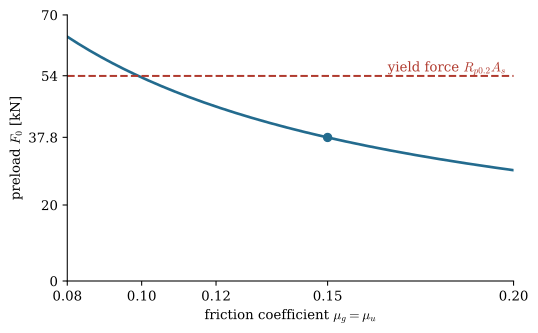
Because friction takes most of the torque, the preload depends on the friction as much as on the torque. Figure 9.6.10 tightens the same bolt to the same 89 N·m with friction coefficients from a well lubricated to a dry thread. The preload ranges from about 30 kN to beyond the yield force of the bolt.
Figure 9.6.10: The preload of the M12 bolt of Example 1 tightened to \(M_t = 89\) N·m, against the friction coefficient. The dot is the design point, \(\mu = 0.15\).
This is why a torque wrench controls the preload only roughly, and why joints that need an accurate preload are tightened by angle after a snug torque, or by measuring the elongation of the bolt. It is also why the friction coefficients deserve care: lubricating a bolt that was specified dry can take it past yield at the specified torque.
The joint under load
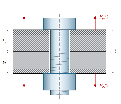
Once tightened, the bolt is a stretched spring and the plates are a compressed one, and both carry the preload \(F_0\). An external tensile load \(F_y\) on the joint, Figure 9.6.11, pulls the plates apart. As long as they stay in contact, the bolt and the plates stretch by the same additional amount \(\delta\). The bolt force rises by \(k_s\delta\), the clamping force between the plates falls by \(k_f\delta\), and together the two changes carry the load, \(k_s\delta + k_f\delta = F_y\), where \(k_s\) and \(k_f\) are the stiffnesses of the bolt and of the plates [2]. With \(\delta = F_y/(k_s + k_f)\) the bolt force and the clamping force are
The joint constant\(C\) is the share of the external load the bolt feels. The plates separate when the clamping force reaches zero, at the external load
and beyond it the bolt carries all of \(F_y\) alone.
Figure 9.6.11: A bolted joint under the external load \(F_y\). The grip \(l = t_1 + t_2\) is the clamped length.
The joint diagram
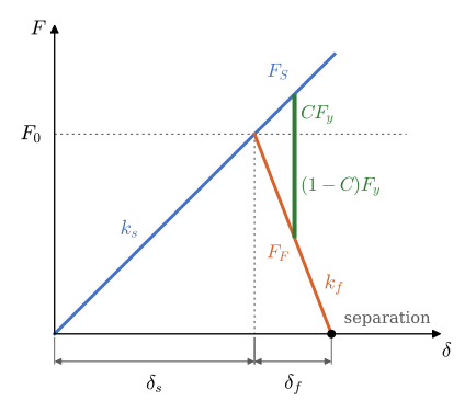
The joint diagram shows 9.6.9 at a glance (Figure 9.6.12). Tightening stretches the bolt along a line of slope \(k_s\) until it carries \(F_0\), an elongation \(\delta_s = F_0/k_s\). The plates are compressed by \(\delta_f = F_0/k_f\) under the same force. Their line is drawn from the end of the bolt line, running down with slope \(-k_f\), so that both share the point \((\delta_s, F_0)\). An external load stretches the joint further: the bolt climbs its line and the plates descend theirs, and the vertical distance between the two lines is \(F_y\). The part above \(F_0\) is the extra bolt force \(CF_y\), the part below is the loss of clamping force \((1 - C)F_y\). Where the plate line meets the axis, the clamping force is gone and the joint opens.
Figure 9.6.12: The joint diagram. The bolt line (slope \(k_s\)) and the plate line (slope \(-k_f\)) meet at the preload \(F_0\). An external load \(F_y\), in green, raises the bolt force to \(F_S\) and lowers the clamping force to \(F_F\).
Stiff plates make the plate line steep and \(C\) small, so most of a fluctuating load only varies the clamping force and the bolt sees a small fraction of it. This is the main reason preload protects a bolt against fatigue. A short, thick bolt does the opposite: it is stiff, \(C\) grows, and the bolt takes much of the load.
Stiffness of the bolt and the plates
The bolt in the grip is a plain shank of area \(A_d = \pi d^2/4\) and length \(l_d\) followed by a threaded part of area \(A_s\) and length \(l_t\). The two carry the same force and add their elongations, so they are springs in series [2],
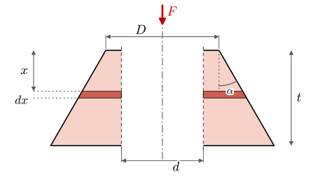
The plates are harder. The clamping force enters them on the bearing ring under the head and the nut and spreads outwards, so only a zone around the bolt is compressed. The usual model takes that zone as a cone widening at the half-angle \(\alpha = 30^\circ\) from the bearing face [2], Figure 9.6.13, the pressure cone of the lecture slides.
(a) The pressure cones in the joint of Example 1
(b) One frustum and its element \(dx\)
Figure 9.6.13: The compressed zone of the plates is modelled as two cones of half-angle \(\alpha\), one from the head and one from the nut, meeting at the joint face.
A slice of the frustum at the depth \(x\) below the bearing face, of thickness \(dx\), is a ring of outer diameter \(D + 2x\tan\alpha\) around the hole of diameter \(d\), with \(D\) the bearing face diameter \(d_w\). Under the force \(F\) it shortens by
and the frustum of thickness \(t\) shortens by the integral of \(d\delta\) from \(0\) to \(t\). Its stiffness \(k = F/\delta\) is, with \(a = \tan\alpha\),
Code
x, t, a, E, Fc = sp.symbols('x t a E F', positive=True) # a = tan(alpha)p, q = sp.symbols('p q', positive=True) # (D + d)/2 and (D - d)/2D_, d_ = sp.symbols('D d', positive=True)delta_cone = Fc/(sp.pi*E)*sp.integrate(1/((a*x + p)*(a*x + q)), (x, 0, t))k_cone = sp.simplify(Fc/delta_cone).subs({p: (D_ + d_)/2, q: (D_ - d_)/2})# the same result in the form of Budynas and Nisbett, Eq. (8-19)k_shigley = sp.pi*E*d_*a/sp.log((2*t*a + D_ - d_)*(D_ + d_)/((2*t*a + D_ + d_)*(D_ - d_)))check = {E: 210000, d_: 12, D_: 16.6, t: 14, a: sp.tan(sp.pi/6)}rel_diff = sp.N((k_cone - k_shigley).subs(check)/k_shigley.subs(check))
\[ k = \dfrac{\pi E a d}{\log{\left(\dfrac{\left(D + d\right) \left(D + 2 a t - d\right)}{\left(D - d\right) \left(D + 2 a t + d\right)} \right)}},\qquad \left|\frac{k_{\text{integral}} - k}{k}\right| = 1\cdot 10^{-16} \]
that is,
\[
k = \frac{\pi E d\tan\alpha}{\ln\dfrac{(2t\tan\alpha + D - d)(D + d)}{(2t\tan\alpha + D + d)(D - d)}}
\tag{9.6.13}\]
the frustum stiffness of Budynas and Nisbett and of the configurator. Each plate is a frustum from its outer face to the joint face, which is exact when the two plates are equally thick and the cones meet there, as in Figure 9.6.13. The plates are in series, \(1/k_f = 1/k_1 + 1/k_2\). A soft gasket in the joint is far less stiff than the steel and then sets \(k_f\) almost alone.
Example 2: The joint under load
The joint of Example 1 has two steel plates of \(t_1 = t_2 = 14\) mm, so the grip is \(l = 28\) mm, and \(E = 210\) GPa for plates and bolt. The bolt is an M12 × 45 with a thread length of 30 mm, so the grip holds \(l_d = 15\) mm of shank and \(l_t = 13\) mm of thread. It is preloaded to \(F_0 = 37.8\) kN and carries the external load \(F_y = 20\) kN. Find the stiffnesses, the joint constant, the bolt and clamping forces and the load at which the plates separate, and draw the joint diagram.
The recipe is 9.6.11 for the bolt, 9.6.13 with \(D = d_w\) for each plate and the series sum for \(k_f\), then 9.6.9 and 9.6.10.
Code
E_st =210e3# MPat1 = t2 =14.0# mml_d, l_t =15.0, 13.0# shank and thread in the grip, mmA_d = np.pi*d**2/4F_y =20e3# Nk_s =1/(l_d/(E_st*A_d) + l_t/(E_st*A_s)) # N/mmdef k_frustum(t, D=d_w, alpha=np.radians(30)): ta = np.tan(alpha)return np.pi*E_st*d*ta/np.log((2*t*ta + D - d)*(D + d)/((2*t*ta + D + d)*(D - d)))k_f =1/(1/k_frustum(t1) +1/k_frustum(t2))C = k_s/(k_s + k_f)F_S = F_0 + C*F_yF_F = F_0 - (1- C)*F_yF_sep = F_0/(1- C)
The stiffnesses, the joint constant and the forces are
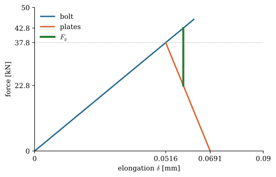
The plates are three times as stiff as the bolt, so the bolt feels a quarter of the external load: 20 kN on the joint raises the bolt force by only 5 kN, while the clamping force drops by 15 kN. The joint stays closed up to \(F_y = 50.6\) kN, and Figure 9.6.14 shows the same numbers as a joint diagram.
Figure 9.6.14: The joint diagram of Example 2. The external load of 20 kN, in green, raises the bolt force from 37.8 to 42.8 kN and lowers the clamping force to 22.8 kN.
If the load varies between zero and 20 kN, the bolt force varies by only \(CF_y = 5\) kN, a stress amplitude of \(CF_y/(2A_s) = 30\) MPa instead of the 119 MPa a bolt without preload would see. The configurator holds joints to the guide that the plates take at least 80 % of the load, \(C \le 0.2\); with \(C = 0.25\) this joint misses it slightly, and a longer grip or a waisted bolt, both lowering \(k_s\), would bring it there.
A short grip in the wind
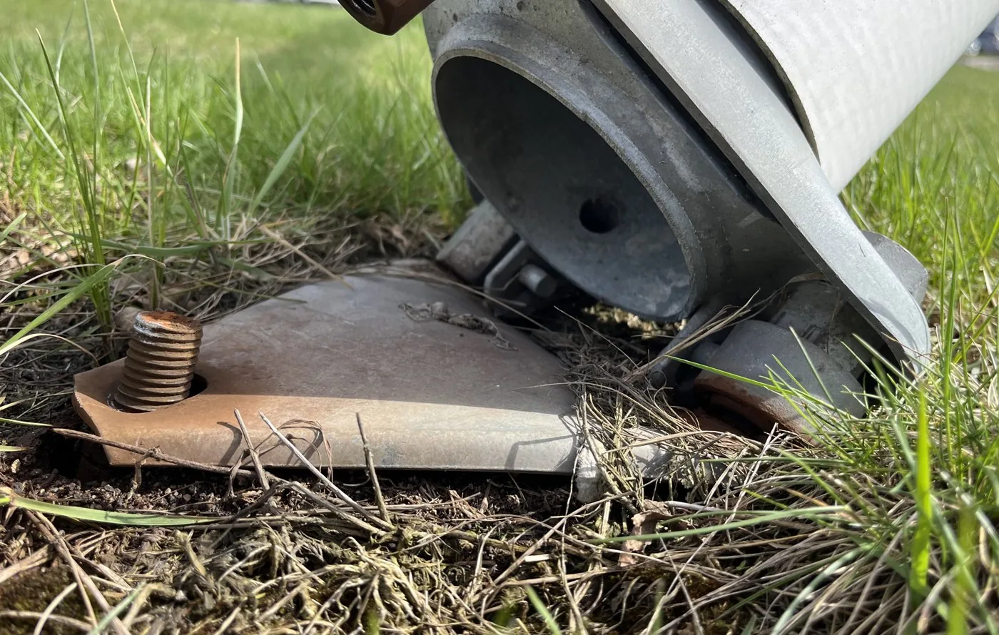
Flagpoles stand in the wind all their lives (Figure 9.6.15). Every gust bends the pole and every swing reverses the bending, so the joint at its foot is loaded in cycles from the day it is put up. The foot of a tilting flagpole is bolted to a base plate in the foundation with nuts on studs, and in Figure 9.6.16 the joint has given way: the pole lies tilted, held only by its hinge, still swinging in the wind.
(a) A pole whose base joint has failed, still swinging on its hinge
(b) A row of poles in the same wind
Figure 9.6.15: Flagpoles in the wind.
(a) The foot of the pole, tilted off the base plate
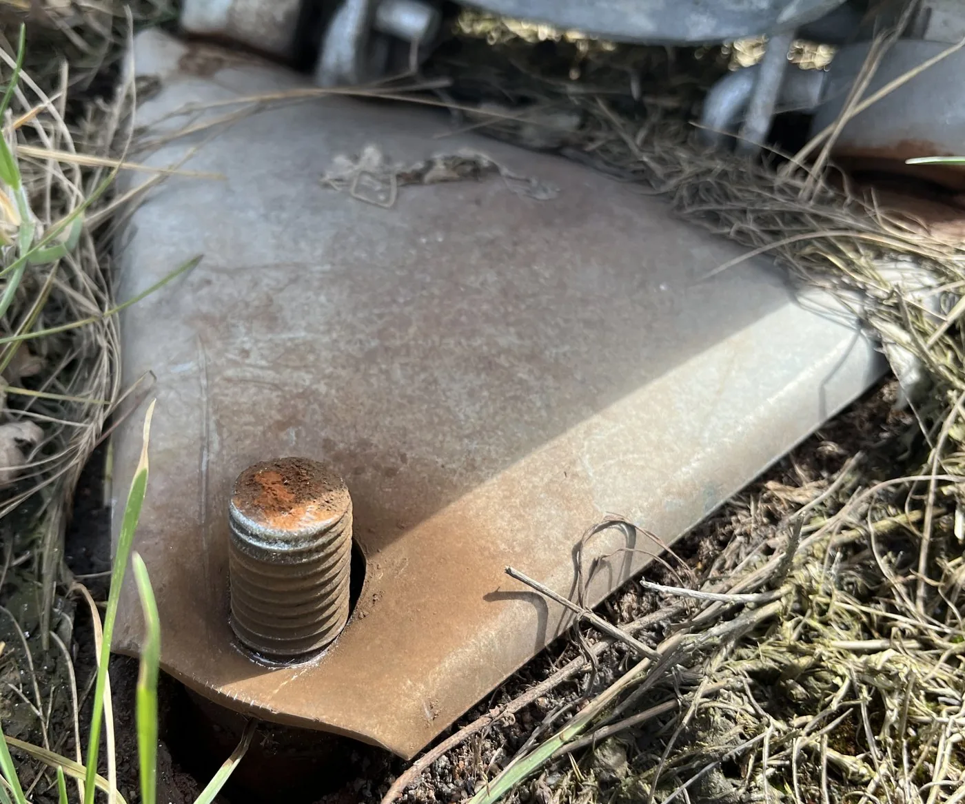
(b) The broken stud in the thin base plate
Figure 9.6.16: The base of the fallen pole. The stud has broken off just above the base plate.
The fracture face of the stud in Figure 9.6.16 (b) is flat and square to its axis, it runs through the root of a thread, and most of it is rusted. That is how a fatigue crack usually looks: it starts at the notch of a thread root, grows a little with each load cycle and rusts as it grows, until the section left over is too small and breaks at once.
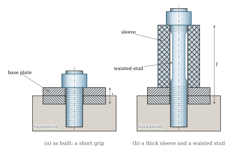
The joint diagram tells us what made the stud sensitive. The nut sat on a thin plate, so the grip was short, the stud between the nut and the foundation was short and stiff, and \(C\) was large: a large share of every gust went straight into the stud. The remedy is to make the flange thick on purpose, Figure 9.6.17. A thick spacer sleeve under the nut makes the clamped stack long and stiff, the stud becomes long, and a waist turned down below the thread root diameter makes it slender as well.
Figure 9.6.17: (a) The nut on a thin base plate gives a short grip. (b) A thick sleeve under the nut and a waisted stud make the grip long, the flange stiff and the bolt slender.
How far this goes follows from 9.6.9. When a length \(L\) of sleeve, of area \(A_\text{sl}\), and the same length of waisted stud, of area \(A_w\), dominate the grip, both stiffnesses are set by \(L\), \(k_s \approx EA_w/L\) and \(k_f \approx EA_\text{sl}/L\), and
\[
C \to \frac{A_w}{A_w + A_\text{sl}}
\tag{9.6.14}\]
The length cancels. What matters is that the sleeve has a much larger area than the stud beside it: a thin tube, no stiffer than the bolt, would only make \(C\) worse.
Example 3: A flagpole base
An M16 stud of class 8.8 clamps an 8 mm base plate onto an 8 mm steel anchor plate in the foundation, and is preloaded to 70 % of its yield force. The wind loads the stud with an external force cycling between 0 and \(F_y = 10\) kN, a value assumed for the example. Compare the stress amplitude in the thread for (a) the nut on the base plate and (b) a steel sleeve of outer diameter 40 mm, inner diameter 17 mm and length 60 mm under the nut, with the stud waisted to 12 mm along the sleeve. The nut has \(d_w = 22.5\) mm.
The recipe is 9.6.11 for the stud, 9.6.13 for each plate, with \(D = d_w\) under the nut in (a) and \(D = 40\) mm under the sleeve in (b), the sleeve as a tube, \(k_\text{sl} = EA_\text{sl}/L\), in series with the plates, then \(C\) from 9.6.9. The bolt force varies by \(CF_y\), so the stress amplitude in the thread is \(\sigma_a = CF_y/(2A_s)\).
Code
d3, A_s3, d_w3 =16, 157.0, 22.5# M16F_03 =0.7*R_p*A_s3 # NF_y3 =10e3# N, cycling 0 -> F_y3t_p =8.0# base plate and anchor plate, mmOD, ID, L_sl, d_waist =40.0, 17.0, 60.0, 12.0def k_cone(t, D, d=d3, alpha=np.radians(30)): ta = np.tan(alpha)return np.pi*E_st*d*ta/np.log((2*t*ta + D - d)*(D + d)/((2*t*ta + D + d)*(D - d)))# (a) nut on the base plate: the stud is threaded through the grip of 2 t_pk_sa = E_st*A_s3/(2*t_p)k_fa =1/(2/k_cone(t_p, d_w3))C_a = k_sa/(k_sa + k_fa)# (b) sleeve under the nut, stud waisted along the sleeveA_sl = np.pi*(OD**2- ID**2)/4A_w = np.pi*d_waist**2/4k_sb =1/(2*t_p/(E_st*A_s3) + L_sl/(E_st*A_w))k_fb =1/(2/k_cone(t_p, OD) + L_sl/(E_st*A_sl))C_b = k_sb/(k_sb + k_fb)sigma_a = C_a*F_y3/(2*A_s3) # MPasigma_b = C_b*F_y3/(2*A_s3)C_lim = A_w/(A_w + A_sl) # the long-sleeve limit
The joint constants and the stress amplitudes in the thread are
\[ \begin{aligned}\text{(a)}\quad C &=0.312,\quad \sigma_a =9.92~\text{MPa}\\ \text{(b)}\quad C &=0.0999,\quad \sigma_a =3.18~\text{MPa},\quad \frac{A_w}{A_w + A_\text{sl}} =0.099\end{aligned} \]
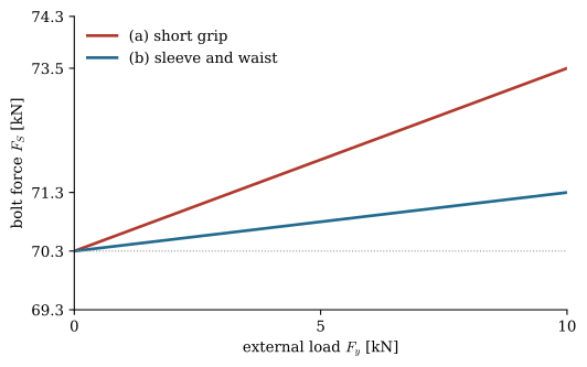
The sleeve and the waist cut the share of the wind load that reaches the stud from 31 % to 10 %, practically the long-sleeve limit of 9.6.14, and the stress amplitude in the thread falls by more than a factor of three. Fatigue life grows steeply as the amplitude falls, typically by far more than the factor on the stress (see the fatigue chapter). The preload is the same in both joints; what changed is only how the external load is shared. Figure 9.6.18 shows the bolt force of both joints over one load cycle.
Figure 9.6.18: The bolt force of the M16 stud of Example 3 as the wind load rises from 0 to 10 kN. Both joints start at the same preload; the short grip passes three times more of the load cycle to the stud.
Embedment
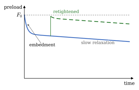
A preload is not kept forever. Seen closely, every contact surface in the joint is rough: under the head, under the nut, between the plates and on the loaded thread flanks. When the bolt is tightened, the highest peaks carry the whole preload and flatten, most of it in the first minutes and hours and in the first load cycles. The joint settles, or embeds, by a small amount \(f_z\), typically a few micrometres for each machined steel surface and more for painted, coated or dirty ones [2]. A slow relaxation follows, from creep and from vibration (Figure 9.6.19).
Figure 9.6.19: The preload over time. Embedment takes a large part of it in the first hours; a joint retightened after the settling keeps a preload close to the one specified.
The settling takes away part of the elongation stored in the joint. The bolt was stretched by \(\delta_s = F_0/k_s\) and the plates compressed by \(\delta_f = F_0/k_f\); after the settling the sum is smaller by \(f_z\), and both lines of the joint diagram move down together, so the preload falls by
A short, stiff joint loses most, the same joint that passes most of a fluctuating load to the bolt. For the joint of Example 2, a settling of only 10 µm costs
The bolt was stretched by only 52 µm, so 10 µm of settling is a fifth of it. This is why a joint that matters is retightened once the settling is over, and why long, slender bolts keep their preload better than short, stiff ones.
Joints loaded in shear
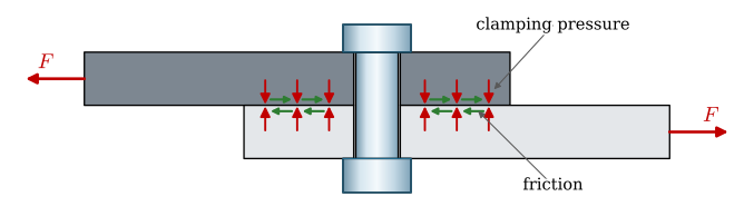
Most bolted joints in machines and structures carry their load across the bolt rather than along it. The bolt then does not act as a pin. The preload presses the plates together, and the friction between them carries the load (Figure 9.6.20). As long as the plates do not slip, the bolt feels nothing but its preload. A joint with \(n_b\) bolts and \(n_f\) friction interfaces carries, before it slips,
The slip factor \(\mu\) depends on the surfaces: design codes for steel structures use values from about \(0.2\) for untreated or oily surfaces to \(0.5\) for blasted steel. Such a slip-resistant joint is designed so that \(F \le F_\text{slip}/S\) with a safety factor \(S\).
Figure 9.6.20: A lap joint in shear. The preload presses the plates together (red), and the friction on each plate (green) holds it against the load \(F\).
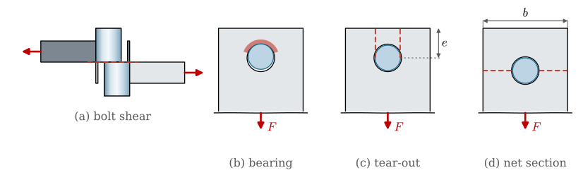
If the load exceeds \(F_\text{slip}\), the plates slide until the edges of the holes meet the bolt, and the bolt is loaded in shear and bending. We consider the joint failed at that point. A joint that has slipped once can slip back and forth under a fluctuating load, loosening the nut and fatiguing the bolt, so slip is the design criterion. The joint then still has strength left as a bearing-type joint, and Budynas and Nisbett list how it fails next [2] (Figure 9.6.21): the bolt shears off, the bolt crushes the edge of the hole, the plate tears out to the edge, or the plate breaks across the hole. With \(F\) per bolt, plate thickness \(t\), bolt diameter \(d\), hole diameter \(d_h\), plate width \(b\) and edge distance \(e\) from the hole centre, the four nominal stresses are
\[
\begin{aligned}
\tau_\text{bolt} &= \frac{F}{A} &\quad &\text{bolt shear, } A = A_d \text{ or } A_r\\
\sigma_b &= \frac{F}{d\,t} & &\text{bearing on the hole (hålkantstryck)}\\
\tau_e &= \frac{F}{2(e - d_h/2)\,t} & &\text{tear-out along two planes to the edge}\\
\sigma_n &= \frac{F}{(b - d_h)\,t} & &\text{tension across the hole}
\end{aligned}
\tag{9.6.17}\]
Tear-out is avoided in practice by keeping the hole centre at least \(1.5d\) from the edge [2].
Figure 9.6.21: Failure of a bearing-type joint: (a) the bolt shears at the interface, (b) the bolt crushes the edge of the hole, (c) the plate tears out along two planes to the edge, (d) the plate breaks across the hole.
Keep the thread out of the shear plane
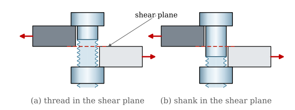
The shear plane of a lap joint is the interface between the plates. If the thread reaches into it (Figure 9.6.22 a), the shear acts on the root area \(A_r = \pi d_3^2/4\), about two thirds of the shank area \(A_d\) for M12 and M16, so the shear stress is half as large again. The thread roots are sharp notches as well, which matters as soon as the load fluctuates, and the crests of the thread bear on the hole edge with a fraction of the contact area of a plain shank. A bolt is therefore chosen long enough for the plain shank to pass through the shear plane, with the thread starting below it (Figure 9.6.22 b). The M12 × 45 bolt of the joint in Example 1 has 15 mm of shank through the 14 mm upper plate for this reason.
Figure 9.6.22: (a) The thread reaches the shear plane: a smaller area, notches and crushed thread crests. (b) The plain shank carries the shear.
Example 4: A lap joint
Two steel plates of S355 (\(R_e = 355\) MPa), 80 mm wide and \(t = 10\) mm thick, overlap and are joined by one M16 bolt of class 8.8 in a 17 mm hole, 30 mm from the plate end. The bolt is preloaded to \(F_0 = 0.7R_{p0.2}A_s\), the slip factor is \(\mu = 0.3\), and the joint carries \(F = 15\) kN. Find the slip load and the load each of the bearing-type failures of 9.6.17 would need, taking yield in tension and \(0.577\) times the yield strength in shear as the limits.
The recipe is 9.6.16 with \(n_f = n_b = 1\), then each line of 9.6.17 solved for the load that brings the stress to its limit.
The joint slips at 21 kN, so it carries 15 kN with a margin of 1.4 against slip. Every other mode needs at least two and a half times as much load, which is why slip, not strength, sets the design of a preloaded shear joint. Had the thread reached the shear plane, the bolt would shear at 53 kN instead of 74 kN.
Two plates and more
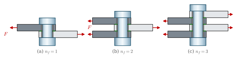
The friction of 9.6.16 acts at every interface the preload presses together. A lap joint of two plates has one (Figure 9.6.23 a). Three plates, a middle plate between two cover plates, have two interfaces for the same bolt and the same preload, so the joint carries twice the load before it slips; the bolt, if it ever bears, is in double shear; and the load path is symmetric, so the plates are not bent as in a single lap. Four interleaved plates have three interfaces. The clamping force is the same at every interface, because it is the same preload passing through the whole stack.
Figure 9.6.23: One bolt through two, three and four plates in tension: one, two and three friction interfaces (green).
Example 5: Three plates instead of two
The 15 kN of Example 4 is now carried by a 10 mm middle plate between two 6 mm cover plates, with the same M16 bolt and preload. With \(n_f = 2\), 9.6.16 gives
twice the slip load of the lap joint, a margin of 2.8 on the same load, with no other change than one more plate.
Flanges under pressure
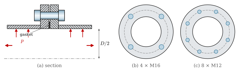
A flanged pipe joint is a tension joint with many bolts (Figure 9.6.24). The pressure \(p\) acts on the area inside the gasket and pushes the two pipe ends apart with \(F_p = p\pi D^2/4\), shared by the \(n\) bolts, so each bolt carries \(F_y = F_p/n\) as the external load of 9.6.9. The gasket seals only while it is pressed, so the clamping force must stay well above zero at full pressure.
Figure 9.6.24: A flanged pipe joint under the internal pressure \(p\). (a) A section through the upper half. (b) and (c) The same flange with four M16 and with eight M12 bolts.
Example 6: Four bolts or eight?
A pipe joint with a gasket diameter \(D = 200\) mm and two 20 mm steel flanges sees a pressure cycling between 0 and 2 MPa. Compare four M16, eight M12 and twelve M10 bolts of class 8.8, each preloaded to 70 % of its yield force, with 30 mm of shank and 10 mm of thread in the 40 mm grip. The three choices have almost the same total stress area.
The total pressure force is \(F_p = 62.8\) kN. For each choice, the total stress area, the joint constant, the stress amplitude in the thread and the total clamping force left on the gasket at full pressure are
With the same steel, more and smaller bolts are better under a cyclic pressure. The smaller bolts are more slender in the same flanges, so \(C\) falls and the stress amplitude with it, and the total clamping force left on the gasket grows. The benefits beyond these numbers point the same way: the pressure cones of closely spaced bolts overlap and press the gasket evenly between the bolts, smaller bolts have a higher fatigue strength for their size, and with twelve bolts the loss of one is a nuisance rather than a failure.
Wheel bolts
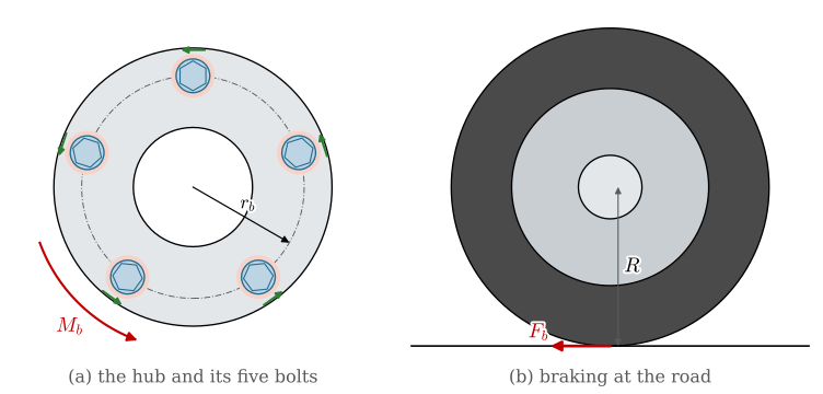
A car wheel is a shear joint too. The brake disc and the hub turn with the wheel, and the braking torque passes from the hub to the rim through friction around each wheel bolt (Figure 9.6.25). The bolts are not pins; they clamp. A wheel bolt seats on a \(60°\) cone in the rim, which centres the wheel and wedges the bolt head into its seat exactly as the thread flank wedges the nut onto the bolt in the flank angle. The normal force on the seat is \(F/\sin 30° = 2F\), so the head friction of 9.6.5 doubles, \(M_u = \mu_u F r_m/\sin 30°\).
Figure 9.6.25: (a) The hub with five wheel bolts on the pitch circle of radius \(r_b\); friction around each bolt (green) carries the braking torque \(M_b\). (b) The braking force \(F_b\) acts at the tyre radius \(R\).
Example 7: Retighten after 100 km
A car of 1500 kg has five M14 × 1.5 wheel bolts on a pitch circle of 112 mm, tightened to \(M_t = 120\) N·m. The friction coefficients are \(\mu_g = \mu_u = 0.14\) in the thread and on the cone seat, whose mean radius is \(r_m = 9\) mm, and an assumed \(0.2\) between rim and hub. In an emergency stop at 1 g, 60 % of the braking acts on the front axle, and the tyre radius is \(R = 0.31\) m. Find the preload, the torque the friction can carry, and what remains of it if a newly fitted wheel settles by \(f_z = 15\) µm, with the bolt stiffness taken as \(E A_s\) over a 30 mm elastic length and the rim and hub as two 10 mm steel frusta from a 21 mm seat.
Code
d7, P7, n7, r_b7 =14.0, 1.5, 5, 56.0# mmd2_7 = d7 -0.6495*P7A_s7 = np.pi/4*((d2_7 + d7 -1.22687*P7)/2)**2mu7, mu_rim, r_m7 =0.14, 0.2, 9.0phi7 = np.arctan(P7/(np.pi*d2_7))rho7 = np.arctan(mu7/np.cos(np.radians(30)))lever7 = d2_7/2*np.tan(phi7 + rho7) + mu7*r_m7/np.sin(np.radians(30)) # cone seatF_07 =120e3/lever7 # N, from M_t = 120 N mM_fr = n7*mu_rim*F_07*r_b7/1e3# N m, friction torque of the wheelM_brake =0.6*1500*9.81/2*0.31# N m, one front wheel at 1 gk_s7 = E_st*A_s7/30.0ta = np.tan(np.radians(30))k_f7 =1/(2/(np.pi*E_st*d7*ta/np.log((2*10*ta +21- d7)*(21+ d7)/((2*10*ta +21+ d7)*(21- d7)))))dF_07 =0.015/(1/k_s7 +1/k_f7)M_fr_settled = n7*mu_rim*(F_07 - dF_07)*r_b7/1e3
The preload, the friction torque against the braking torque, before and after the settling, are
Freshly tightened, the friction carries the hardest stop with a margin of about 30 %. The cone seat costs a lot of that preload: with a flat seat the same 120 N·m would give half as much again. After 15 µm of settling, which paint, rust, dirt or an aluminium rim on a new contact can easily give, a third of the preload is gone and the friction torque falls below the braking torque. The wheel can then shift on the hub in a hard stop, the bolts take the load in shear and bending, and every stop and start works them looser. This is why the tyre shop asks us to retighten the bolts after the first 100 km: the settling is over by then, and retightening restores the preload, Figure 9.6.19.
The bolted joint configurator
The configurator computes 9.6.6 and 9.6.7 for the coarse metric threads from M3 to M30, with friction coefficients chosen from the surface treatment and the lubrication of the bolt and the nut, and continues with 9.6.11, 9.6.13 and the joint diagram for flanges of any thickness and material.
The numbers are chosen so that each problem can be worked with the equations of the chapter and a calculator. Each answer is blurred until the mouse rests on it, or it is tapped.
Problem 1: Lubricated threads. An M10 bolt of class 8.8 (\(P = 1.5\) mm, \(d_2 = 9.026\) mm, \(A_s = 58.0\) mm²) is to be preloaded to 70 % of its yield force. The bearing face has \(d_w = 14.6\) mm and the hole \(d_h = 11\) mm, and the bolt is lubricated, \(\mu_g = \mu_u =
0.10\). Find the tightening and the loosening torque. The drawing specifies the torque for a dry bolt, \(\mu = 0.15\); what preload does that torque give when applied to the lubricated bolt?
Figure 9.6.26: The bolt of Problem 1 is an M10 of the same pattern as this M12.
Answer:\(F_0 = 26.0\) kN, \(M_t = 36.5\) N·m, \(M_l = 23.9\) N·m. The dry torque is 51.7 N·m and gives the lubricated bolt 36.8 kN, 99 % of its yield force of 37.1 kN.
Problem 2: Aluminium plates. An M10 steel bolt clamps two aluminium plates (\(E = 70\) GPa), each 12 mm thick, as in Figure 9.6.27. The grip holds 14 mm of shank and 10 mm of thread, and \(d_w = 14.6\) mm. The preload is 25 kN. Find \(k_s\), \(k_f\), \(C\), the bolt force under an external load of 10 kN, and the load at which the plates separate.
Figure 9.6.27: The joint of Problem 2, with \(t_1 = t_2 = 12\) mm.
Answer:\(k_s = 599\) kN/mm, \(k_f = 674\) kN/mm, \(C = 0.47\), \(F_S = 29.7\) kN, separation at \(47.2\) kN. The soft plates pass almost half of the load to the bolt.
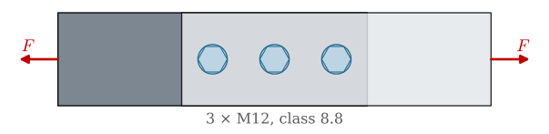
Problem 3: Three bolts in a lap joint. Two plates are joined by three M12 bolts of class 8.8, each preloaded to 70 % of its yield force (Figure 9.6.28). The slip factor is \(\mu = 0.3\). Find the largest load \(F\) the joint can carry with a safety factor of 1.5 against slip.
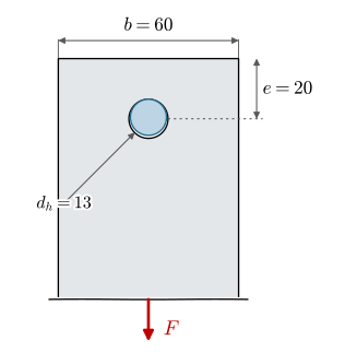
Problem 4: A bearing-type joint. An 8 mm plate of S235 (\(R_e = 235\) MPa), 60 mm wide, is held by one M12 bolt without preload in a 13 mm hole whose centre is 20 mm from the end (Figure 9.6.29). It carries \(F = 20\) kN. Find the shear stress in the shank, the bearing stress, the tear-out stress and the net-section stress, and which of them limits the load if \(F\) grows, with the limits of Example 4.
Figure 9.6.29: The plate end of Problem 4.
Answer:\(\tau = 177\) MPa, \(\sigma_b = 208\) MPa, \(\tau_e = 93\) MPa, \(\sigma_n = 53\) MPa. Bearing limits first, at 22.6 kN, before tear-out at 29.3 kN, bolt shear at 41.8 kN and the net section at 88 kN. The edge distance of 20 mm just meets the rule \(e \ge 1.5d = 18\) mm.
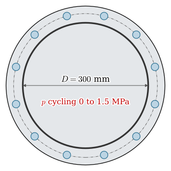
Problem 5: A pressure vessel lid. A lid with a gasket diameter of 300 mm closes a vessel whose pressure cycles between 0 and 1.5 MPa (Figure 9.6.30). It is held by M16 bolts of class 8.8, preloaded to 60 kN, with \(C = 0.2\). How many bolts are needed for the stress amplitude in the thread to stay below 10 MPa, and what clamping force does each keep at full pressure?
Problem 6: A small car. A small car has four wheel bolts on a 100 mm pitch circle, each preloaded to 30 kN, and a friction coefficient of 0.2 between rim and hub (Figure 9.6.31). The tyre radius is 0.29 m. What braking force can one wheel take before the rim slips on the hub?
Figure 9.6.31: The wheel of Problem 6 has four bolts instead of five.
Budynas and Nisbett [2, Ch. 8] derive the thread and collar moments for power screws and bolts, and give measured scatter of the preload at a given torque. Björk [1] collects the formulas and the friction coefficients used here in the form Swedish engineers look them up. The Efficient Engineer’s video The Incredible Strength of Bolted Joints tells the story of preload, from the joint types to the ways of controlling it, and his follow-up on joint diagrams builds the diagram of Figure 9.6.12 step by step.
References
[1]
Björk K. Formler och tabeller för mekanisk konstruktion. 9th ed. Spånga: Karl Björks förlag HB; 2022.