“En tout équilibre de forces quelconques, … la somme des Energies affirmatives sera égale à la somme des Energies négatives prises affirmativement.”
“In every equilibrium of any forces whatever, … the sum of the positive energies will be equal to the sum of the negative energies taken as positive.”
— Johann Bernoulli, letter to Pierre Varignon, 26 January 1717, printed in Varignon, Nouvelle mécanique ou statique, 1725
The last example of Work, energy and power found the moment on the screw of a testing machine from the work done in one turn, without a single force inside the machine. The same shortcut shows up when a mechanism’s input moment is computed as a force times the derivative of a length with respect to an angle, \(M = F\,dx/d\theta\). It gives the right number, and this chapter explains why. Comparing the work of the forces for a small imagined motion of the mechanism, a virtual displacement, gives the equilibrium equation directly, and every pin, guide and support drops out of it.
The principle reaches further than mechanisms. It decides whether an equilibrium is stable, it defines the generalised force of a coordinate, and with d’Alembert’s principle it gives the equations of motion of a dynamic system without its reactions, which the Euler-Lagrange equations build on. In Energy methods the same principle, applied to deformable bodies, becomes the starting point of the finite element method.
Virtual displacements
A virtual displacement\(\delta\bm r\) is a displacement we imagine, not one that happens. It is infinitesimally small. It is allowed by the constraints: a pinned point does not move, a point on a guide moves along the guide, and the bodies of a mechanism stay connected. It is taken with time frozen, so every force keeps its present value while we imagine it. Apart from that it is arbitrary, and the principle below must hold for every such displacement.
A real displacement \(d\bm r = \bm v\,dt\) happens in the time \(dt\) and follows the motion. A virtual displacement needs no time and no motion: a mechanism at rest has as many virtual displacements as it has degrees of freedom. The symbol \(\delta\) obeys the rules of the differential \(d\), so for a position that depends on an angle, \(\delta x = (dx/d\theta)\,\delta\theta\) and \(\delta(\sin\theta) = \cos\theta\,\delta\theta\).
The work of a force \(\bm F\) through the virtual displacement \(\delta\bm r\) of its point of application, and of a moment \(M\) through a virtual rotation \(\delta\theta\), is the virtual work
\[
\delta U = \bm F\cdot\delta\bm r , \qquad \delta U = M\,\delta\theta .
\]
The principle of virtual work
For a particle, the virtual work of all forces is \(\delta U = \bigl(\sum\bm F\bigr)\cdot\delta\bm r\). If the particle is in equilibrium, \(\sum\bm F = \bm 0\) and \(\delta U = 0\) for every \(\delta\bm r\). The converse also holds: if \(\delta U = 0\) for every \(\delta\bm r\), choosing \(\delta\bm r\) along \(\bm e_x\) and then along \(\bm e_y\) shows that both components of \(\sum\bm F\) vanish.
A rigid body has the virtual displacements of a rigid body: a translation \(\delta\bm r_G\) and a rotation \(\delta\theta\), so that a point \(P\) moves by \(\delta\bm r_P = \delta\bm r_G + \delta\theta\,\bm e_z\times\bm r_{GP}\). Summing the virtual work of all forces on the body,
which vanishes for every \(\delta\bm r_G\) and \(\delta\theta\) exactly when \(\sum\bm F = \bm 0\) and \(\sum M_G = 0\). The principle of virtual work is the equilibrium of statics in another form:
A system is in equilibrium if and only if the virtual work of all forces on it is zero for every virtual displacement.
Forces that do no virtual work
The principle is useful because of the forces that drop out of it. A reaction does no virtual work when its point of application cannot move along it in any virtual displacement the constraints allow. That holds for a fixed pin, whose point does not move; for a smooth guide or surface, whose normal force is perpendicular to every allowed \(\delta\bm r\); and for a wheel rolling without slip, whose contact point is momentarily at rest. Between two bodies of a mechanism, a pin applies equal and opposite forces to two points that move by the same \(\delta\bm r\), so their virtual work cancels, and the same holds for a rigid link or an inextensible rope. Constraints with this property are called ideal.
For a system of rigid bodies connected by ideal constraints, \(\delta U\) therefore contains only the active forces: applied loads and moments, weights, spring and damper forces, and friction. Meriam and Kraige draw them in an active-force diagram, a sketch of the whole system with only these forces on it, which replaces the free body diagram of every part.
The number of independent virtual displacements is the number of degrees of freedom. A mechanism with one degree of freedom has all its virtual displacements fixed by a single one, \(\delta q\), and \(\delta U = Q\,\delta q = 0\) for every \(\delta q\) is one equation, \(Q = 0\), with no reactions in it.
Example 1: The moment on a crank
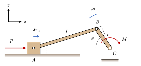
We return to the crank-slider of Example 11 in Particle kinematics, with the crank \(OB\) of length \(r = 125\) mm, the connecting rod \(AB\) of length \(L = 350\) mm and the slider \(A\) moving on the line through \(O\) (Figure 7.8.1). The gas in a cylinder pushes the slider towards \(O\) with the force \(P = 5\) kN. Find the moment \(M\) on the crank that holds the mechanism in equilibrium, as a function of the crank angle \(\theta\). The parts are light, and the joints and the guide are frictionless.
Figure 7.8.1: The crank-slider with the piston force \(P\) and the crank moment \(M\), drawn positive in the sense of increasing \(\theta\), which turns the crank clockwise. The dashed outline is the mechanism after the virtual rotation \(\delta\theta\); the slider has moved by \(\delta x_A\).
Step 1 - Virtual work
The mechanism has one degree of freedom, the crank angle \(\theta\). The active forces are \(P\) and \(M\); the bearing at \(O\), the three pins and the guide of the slider are ideal and do no virtual work. The position of the slider is known from the kinematics chapter,
so a virtual rotation \(\delta\theta\) moves the slider by \(\delta x_A = (dx_A/d\theta)\,\delta\theta\). The piston force points in \(+x\) and does the work \(P\,\delta x_A\); the moment does \(M\,\delta\theta\). The principle of virtual work requires
\[
\delta U = M\,\delta\theta + P\,\frac{dx_A}{d\theta}\,\delta\theta = 0
\quad\text{for every }\delta\theta
\quad\Longrightarrow\quad
M = -P\,\frac{dx_A}{d\theta} .
\tag{7.8.1}\]
This is the “force times the derivative of a length” rule, with its sign and its conditions: it holds for an ideal mechanism in equilibrium, or moving so slowly that the inertia of its parts does not count.
Code
th, r, L, P = sp.symbols('theta r L P', positive=True)x_A =-(r*sp.cos(th) + sp.sqrt(L**2- r**2*sp.sin(th)**2))M_vw = sp.simplify(-P*sp.diff(x_A, th))M_hand =-P*r*sp.sin(th)*(1+ r*sp.cos(th)/sp.sqrt(L**2- r**2*sp.sin(th)**2))hand_check = sp.simplify(M_hand - M_vw)
Differentiating \(x_A\) and collecting the terms gives the moment, checked against the derivative computed directly,
\[ \begin{aligned}M &=- P r \left(\dfrac{r \cos{\left(\theta \right)}}{\sqrt{L^{2} - r^{2} \sin^{2}{\left(\theta \right)}}} + 1\right) \sin{\left(\theta \right)}\\ M - \left(-P\frac{dx_A}{d\theta}\right) &=0\end{aligned} \]
Step 2 - The same moment from free body diagrams
The free body diagrams give the same result with more unknowns. The rod \(AB\) is a two-force member and carries a force \(S\) along its axis \(\bm e_{AB}\). Equilibrium of the slider along the guide, \(P + S\,\bm e_{AB}\cdot\bm e_x = 0\), gives \(S\). The rod then pulls on the crank at \(B\) with \(-S\bm e_{AB}\), and moment equilibrium of the crank about \(O\) gives \(M\). Since increasing \(\theta\) turns the crank clockwise, \(M\) in the sense of \(\theta\) balances the anticlockwise moment of the rod force,
\[
M = \bigl(\bm r_{OB}\times(-S\,\bm e_{AB})\bigr)\cdot\bm e_z .
\]
The guide force, the reaction at \(O\) and the force in the rod appear on the way and are not wanted.
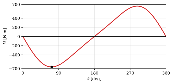
The moment is negative over the first half turn: there the piston pushes the crank towards larger \(\theta\), and the holding moment acts against it. Its magnitude is largest, 664 N·m, at \(\theta \approx 72^\circ\), more than the \(Pr = 625\) N·m a force on a lever of length \(r\) would give, because the inclined rod adds to the lever. Over the second half turn the piston pushes the other way and the sign changes. At \(\theta = 0\) and \(180^\circ\) the crank and the rod lie on one line, \(dx_A/d\theta = 0\), and the piston force cannot turn the crank whatever its size. These are the dead centres, and an engine passes them on the energy stored in its flywheel.
7.8.1 is also a power balance. With \(\dot x_A = (dx_A/d\theta)\,\omega\), multiplying it by \(\omega\) gives \(M\omega = -P\dot x_A\): the power at the crank equals the power at the piston. The slider velocity plotted in the kinematics chapter is the same curve, scaled by \(-P/\omega\).
Example 2: A scissor lift
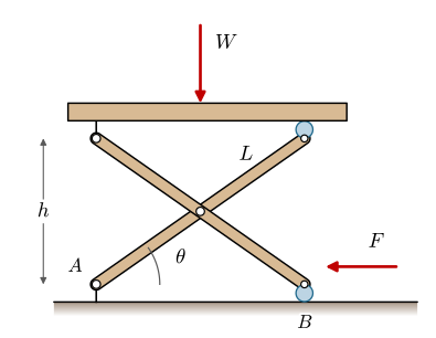
A scissor lift raises a platform with two bars of length \(L = 1.2\) m, pinned together at their midpoints (Figure 7.8.2). One bar is pinned to the ground at \(A\) and carries the platform on a roller; the other is pinned to the platform and runs on a roller at \(B\) on the ground. A horizontal actuator pulls the roller \(B\) towards \(A\) with the force \(F\). The platform carries the load \(W = 3\) kN, its own weight included; the bars are light and the joints frictionless. Find \(F\) as a function of the angle \(\theta\) of the bars.
Figure 7.8.2: A one-stage scissor lift. The bars of length \(L\) make the angle \(\theta\) with the ground; the platform carries the load \(W\) and the actuator pulls the roller \(B\) with \(F\).
Step 1 - Virtual work
The lift has one degree of freedom, \(\theta\). The height of the platform and the position of the roller are
so a virtual change \(\delta\theta\) raises the platform by \(\delta h = L\cos\theta\,\delta\theta\) and moves the roller by \(\delta x_B = -L\sin\theta\,\delta\theta\). The load points down and does \(-W\delta h\); the actuator force points in \(-x\) and does \(-F\delta x_B\). All pins and rollers are ideal, so
\[
\delta U = -W L\cos\theta\,\delta\theta + F L\sin\theta\,\delta\theta = 0
\quad\Longrightarrow\quad
F = \frac{W}{\tan\theta} .
\tag{7.8.2}\]
Step 2 - The free body diagrams, for comparison
Cutting the lift into its three parts, the two bars and the platform, gives nine equations of equilibrium. Their unknowns are the two components of the pin force at \(A\), the roller force at \(B\), the two components of the force in the middle pin, the two components at the platform pin, the platform roller force, and \(F\). Virtual work needed one equation for \(F\); the free body diagrams need all nine.
Code
th2, Ls, W = sp.symbols('theta L W', positive=True)Ax, Ay, By, Ex, Ey, Cx, Cy, Dy, F = sp.symbols('A_x A_y B_y E_x E_y C_x C_y D_y F', real=True)c, s = sp.cos(th2), sp.sin(th2)pA, pB = sp.Matrix([0, 0]), sp.Matrix([Ls*c, 0])pC, pD, pE = sp.Matrix([0, Ls*s]), sp.Matrix([Ls*c, Ls*s]), sp.Matrix([Ls*c/2, Ls*s/2])pW = sp.Matrix([Ls*c/2, Ls*s])def moment(p, f): # moment about A of the force f acting at preturn p[0]*f[1] - p[1]*f[0]bar_AD = [(pA, sp.Matrix([Ax, Ay])), (pE, sp.Matrix([Ex, Ey])), (pD, sp.Matrix([0, -Dy]))]bar_BC = [(pB, sp.Matrix([-F, By])), (pE, sp.Matrix([-Ex, -Ey])), (pC, sp.Matrix([-Cx, -Cy]))]platform = [(pC, sp.Matrix([Cx, Cy])), (pD, sp.Matrix([0, Dy])), (pW, sp.Matrix([0, -W]))]eqs9 = []for body in (bar_AD, bar_BC, platform): eqs9 += [sum(f[0] for _, f in body), sum(f[1] for _, f in body), sum(moment(p, f) for p, f in body)]F_fbd = sp.simplify(sp.solve(eqs9, [Ax, Ay, By, Ex, Ey, Cx, Cy, Dy, F], dict=True)[0][F])
Solved together, the nine equations give the actuator force
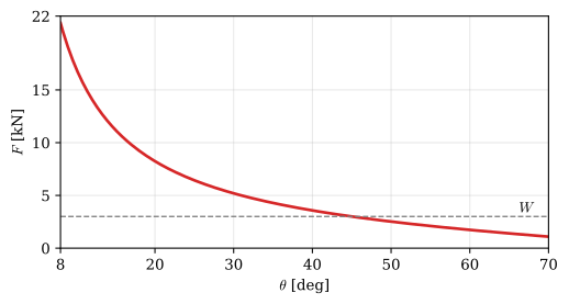
which is 7.8.2. The force grows without bound as the lift folds flat: at \(\theta = 10^\circ\) the actuator must pull with 17 kN to hold 3 kN. Scissor lifts therefore start from an angle well above zero, or push their actuator at an angle to the ground, which a second virtual work calculation would size. With \(n\) stages stacked, \(h = nL\sin\theta\) and the force becomes \(F = nW/\tan\theta\).
Friction is an active force: it does work, and it does not drop out. Its virtual work needs the normal force at the contact, which only a free body diagram gives, and its direction depends on the direction of the motion, so a mechanism with friction has different equilibrium forces for raising and for lowering a load. In practice friction enters through the efficiency of Work, energy and power. A machine driven forward delivers only the fraction \(\eta\) of its input work at the output, so the input force or moment from an ideal virtual work calculation is divided by \(\eta\). For the crank-slider driven by its crank against the piston, \(M = -P\,(dx_A/d\theta)/\eta\); for the screw of the testing machine, the work balance per turn \(\eta_s\,2\pi M_s = Fp\) was exactly this.
Potential energy and stability
When the active forces are conservative, their virtual work is the decrease of their potential energy, \(\delta U = -\delta V\), as in Work, energy and power. For a system with one degree of freedom \(q\), \(\delta V = (dV/dq)\,\delta q\), and the principle of virtual work becomes
\[
\frac{dV}{dq} = 0 .
\]
An equilibrium is a point where the potential energy is stationary. Whether it is stable depends on what happens when the system is nudged. At a minimum of \(V\), any displacement raises the energy, which the system has to be given, and it returns; at a maximum, a displacement releases energy and the system moves on. The test is the second derivative,
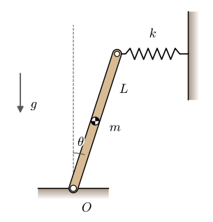
A uniform bar of mass \(m = 10\) kg and length \(L = 1\) m stands on a pin \(O\) and is held at its top by a spring of stiffness \(k\) (Figure 7.8.3). The far end of the spring slides on a vertical guide at the wall, so the spring stays horizontal, and it is unstretched when the bar is vertical. For which stiffness is the vertical position stable?
Figure 7.8.3: The bar on the pin \(O\) leans by \(\theta\) from the vertical; the horizontal spring at its top stretches by \(L\sin\theta\).
The spring stretches by \(L\sin\theta\) and the centre of mass sits at the height \(\tfrac{L}{2}\cos\theta\) above the pin, so the potential energy is
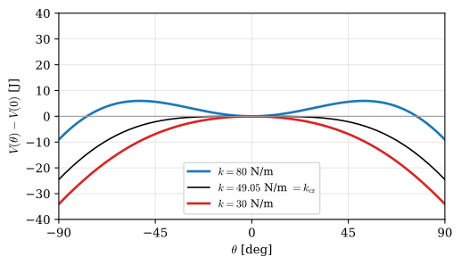
With \(k = 80\) N/m the energy has a minimum at \(\theta = 0\) and the bar, nudged, returns to the vertical. The minimum is local: beyond the maxima at about \(\pm 50^\circ\) the weight wins even over this spring, so the bar is stable against small disturbances, not against any lean. With \(k = 30\) N/m the vertical is a maximum: the spring is too weak to hold the bar, and any lean grows until the bar falls. The critical stiffness separates the two. The same reasoning, with a column for the bar and its bending stiffness for the spring, gives the critical load of Buckling.
Generalised coordinates and generalised forces
The crank angle, the angle of the scissor bars and the lean of the bar each fixed the position of a whole system. A coordinate that does so is a generalised coordinate\(q\), and the virtual work of the active forces for a virtual change \(\delta q\) defines the generalised force\(Q\),
where \(\bm r_i\) is the point where the force \(\bm F_i\) acts and \(\theta_j\) the angle of the body the moment \(M_j\) acts on. When \(q\) is a length, \(Q\) is a force; when \(q\) is an angle, \(Q\) is a moment. The two are the work-conjugate pairs of Work, energy and power. For the crank-slider \(Q = M + P\,dx_A/d\theta\), and \(M = F\,dx/d\theta\) is the statement \(Q = 0\). For conservative forces \(Q = -dV/dq\), and a system with several degrees of freedom has one generalised force for each coordinate.
TipIn industry: robot force control uses virtual work
A robot that presses a tool against a workpiece with the force \(\bm F\) needs the joint moments \(\bm\tau = \bm J^\mathsf{T}\bm F\), where the Jacobian \(\bm J\) maps small joint rotations to small tool displacements, \(\delta\bm x = \bm J\,\delta\bm q\). This is the principle of virtual work, \(\bm\tau^\mathsf{T}\delta\bm q = \bm F^\mathsf{T}\delta\bm x\) for every \(\delta\bm q\). The transpose of a Jacobian returns in How a motion solver works, where it carries the joint reactions.
d’Alembert’s principle
Newton’s second law, written as \(\bm F - m\bm a = \bm 0\), is an equilibrium of the force \(\bm F\) and the inertia force\(-m\bm a\). Jean le Rond d’Alembert made this the basis of dynamics in 1743, and with it the principle of virtual work carries over from statics to motion:
For a rigid body the inertia terms are those of the kinetic diagram in Rigid body kinetics, and 7.8.3 reads \(\bigl(\sum\bm F - m\bm a_G\bigr)\cdot\delta\bm r_G + \bigl(\sum M_G - \bar I\alpha\bigr)\delta\theta = 0\). The ideal constraints still do no virtual work, so their reactions drop out of the dynamics as they did from the statics: each degree of freedom gives one equation of motion, with no reactions in it. Virtual displacements are taken with time frozen, so they are the same in the dynamic problem as in the static one.
Example 4: The collar once more
The collar of Example 1 in Work, energy and power slides on its circular guide under its weight and the spring force, and the guide pushes on it with the normal force \(N\) (Figure 7.3.2). The collar has one degree of freedom, \(\theta\). Its position is \(\bm r_C = -r\bm e_n\), so a virtual rotation moves it along the guide,
\[
\delta\bm r_C = r\,\bm e_t\,\delta\theta .
\]
The normal force is perpendicular to \(\delta\bm r_C\) and drops out. With the acceleration \(\bm a = r\ddot\theta\,\bm e_t + r\dot\theta^2\,\bm e_n\), 7.8.3 gives
the tangential equation of Example 1, obtained without writing the normal force down. The normal equation, which gave \(N\), has no virtual displacement to go with it: a virtual displacement off the guide is not allowed. That is the price of the method. It gives the motion and none of the reactions, which then come from Newton’s second law afterwards, as \(N\) did.
Setting the virtual work to zero and comparing with 7.3.1,
\[ \begin{aligned}\ddot\theta_{\text{d'Alembert}} &=\dfrac{- \dfrac{d^{2} k \sin{\left(\theta \right)}}{\sqrt{d^{2} + 2 d r \cos{\left(\theta \right)} + r^{2}}} + d k \sin{\left(\theta \right)} + g m \cos{\left(\theta \right)}}{m r}\\ \ddot\theta_{\text{d'Alembert}} - \ddot\theta_{\text{Newton}} &=0\end{aligned} \]
From here
The Euler-Lagrange equations take the virtual displacement \(\delta q\) of this chapter, write the inertia term through the kinetic energy and the conservative forces through the potential energy, and give the equations of motion of a system with several degrees of freedom from two scalar functions. The pendulum on the cart of Rigid body kinetics, five equations with Newton-Euler, becomes two.
Energy methods applies the principle to bodies that deform. A virtual displacement then also strains the material, the stresses do internal virtual work, and requiring internal and external virtual work to be equal for every virtual displacement is the starting point of the finite element method.
Further reading
Meriam and Kraige treat virtual work for systems with one degree of freedom, with the active-force diagram, mechanical efficiency and potential energy stability, in chapter 7 of their Statics[1], with many problems.