“It was apparent that the satisfaction of these three fundamental equations proved convergence to the exact elasticity solution as the mesh was refined.”
— Ray W. Clough and Edward L. Wilson, Early Finite Element Research at Berkeley, 1999
The continuum model of Chapter 8.9 rests on three relations and nothing else. Equilibrium 8.7.8 connects the load to the stress, the kinematic definition 8.7.3 connects the displacement to the strain, and the constitutive law 8.9.7 connects the strain to the stress. Every problem in solid mechanics is those three, closed by boundary conditions.
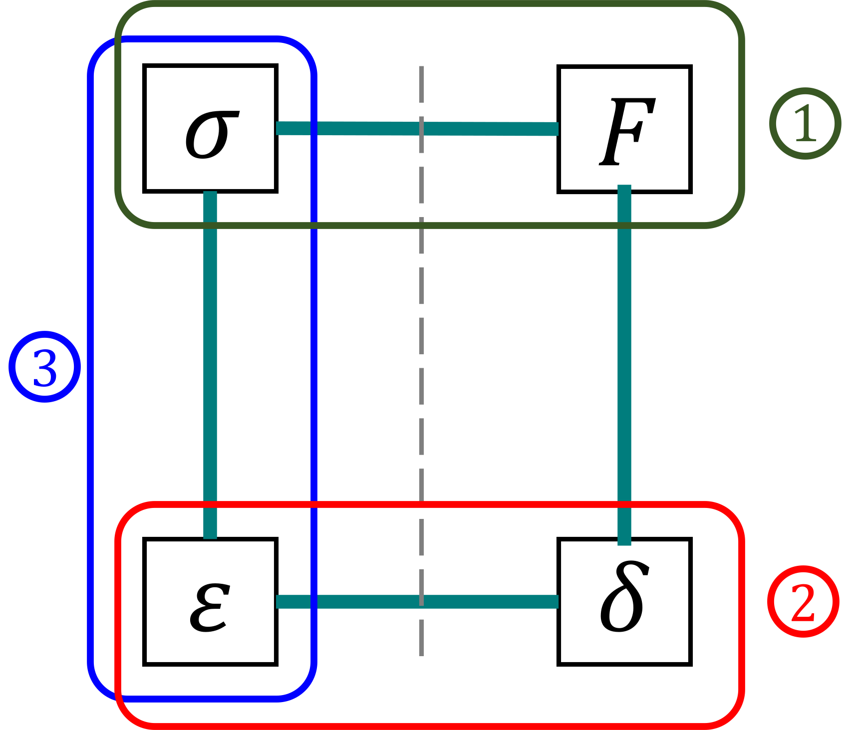
That structure is worth naming, because it survives the reduction to one dimension intact and it tells us what to write down before we know how to solve anything. We call the picture the Golden Quad.
Figure 8.11.1: The Golden Quad. External quantities on the right, internal on the left, joined by the three relations.
On the right sit the external quantities, the load \(F\) and the deformation \(\delta\), which are what a customer specifies and what an instrument measures. On the left sit the internal quantities, the stress \(\sigma\) and the strain \(\varepsilon\), which live inside the material and decide whether it survives. Three relations connect the four corners.
Equilibrium connects the load to the stress. These come from mechanics: a cut, a free body diagram and \(\sum F_i = 0\). In the continuum they are 8.7.8 and 8.7.9; in one dimension they collapse to
\[
\boxed{\sigma = N/A}.
\tag{8.11.1}\]
Deformation relations, also called kinematic relations, connect the deformation to the strain. They are purely geometric and contain no physics at all. In the continuum they are 8.7.3; in one dimension they are
\[
\boxed{\delta = L\varepsilon}.
\tag{8.11.2}\]
Boundary conditions almost always enter here, since what we know about a support is usually a statement about displacement.
Material relations, also called constitutive relations, connect the strain to the stress. Unlike the other two they cannot be derived and must be measured, which is what Chapter 8.6 was about. In the continuum they are 8.9.7, in one dimension
\[
\boxed{\sigma = E\varepsilon},
\tag{8.11.3}\] and thermal effects enter here through
The Golden Quad prescribes a two-step method that separates the part of the work that requires an engineer from the part that does not.
The first step is to write down every relation in Figure 8.11.1 for the problem at hand, one equation at a time, without eliminating anything. Choosing which cuts to make, which supports constrain what, and which material model applies is the mechanics, and it is where modelling judgment lives.
The second step is to solve the resulting system. This is not mechanics. It is algebra, it is mechanical, it is where hand calculations go wrong, and it belongs to the computer. We therefore never eliminate unknowns by substitution on paper. We collect the equations in a list and hand them to SymPy.
⚠ Note
Count equations and unknowns before solving. The Golden Quad tends to produce more unknowns than a first reading of the problem suggests, and a system with the wrong count is a modelling error, not an algebra error.
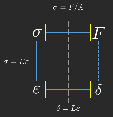
Applied to a rod in simple tension, the three relations are one line each,
which is the elementary formula for the elongation of a bar. The group \(EA\) is the axial stiffness, the counterpart of the bending stiffness \(EI\) of 8.16.9, and \(EA/L\) is the spring constant of the bar.
Figure 8.11.2: The Golden Quad for a rod in simple tension, with all three relations filled in.
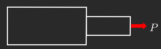
For bodies in series the same force passes through each and the deformations add,
Figure 8.11.3: Bodies in series carry the same force and their deformations add.
Example 1: A heated rod between rigid walls
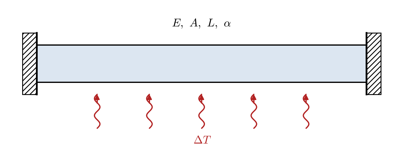
A linear elastic rod is fastened between two rigid walls and then heated by \(\Delta T\). Determine the stress in the rod and the force it exerts on the walls.
Figure 8.11.4: A rod restrained between two rigid walls.
No external load is applied, which makes this a problem that pure statics cannot touch: equilibrium alone gives \(N = P\) and stops. The extra information comes from the deformation relation, because the walls impose \(\delta = 0\) while the material wants to expand.
Figure 8.11.5: Cut and free body diagram.
Writing down all five relations without eliminating anything gives
which is seven equations in the seven unknowns \(N\), \(P\), \(\sigma\), \(\delta\), \(\varepsilon_{\text{tot}}\), \(\varepsilon_{\text{elast}}\) and \(\varepsilon_T\).
N, P, sigma, delta = sp.symbols('N P sigma delta', real=True)eps_tot, eps_el, eps_T = sp.symbols('varepsilon_tot varepsilon_elast varepsilon_T', real=True)E, A, L, alpha, dT = sp.symbols('E A L alpha Delta_T', real=True)eqs = [sp.Eq(N - P, 0), sp.Eq(sigma, N/A), sp.Eq(eps_tot, delta/L), sp.Eq(delta, 0), sp.Eq(sigma, E*eps_el), sp.Eq(eps_T, alpha*dT), sp.Eq(eps_tot, eps_el + eps_T)]sol = sp.solve(eqs, [N, P, sigma, delta, eps_tot, eps_el, eps_T], dict=True)[0]sol | la
\[ \begin{aligned}
N &= - A \Delta_{T} E \alpha \\[9.0pt]
P &= - A \Delta_{T} E \alpha \\[9.0pt]
\delta &= 0 \\[9.0pt]
\sigma &= - \Delta_{T} E \alpha \\[9.0pt]
\varepsilon_{T} &= \Delta_{T} \alpha \\[9.0pt]
\varepsilon_{elast} &= - \Delta_{T} \alpha \\[9.0pt]
\varepsilon_{tot} &= 0
\end{aligned} \]
The rod pushes on the walls with \(P = -EA\alpha\Delta T\) and carries a stress \(\sigma = -E\alpha\Delta T\). Both are negative for a positive temperature change, which is right: heating a rod that cannot expand puts it in compression. A dimensional check passes, since \(E\alpha\Delta T\) has the units of \(E\).
The magnitude deserves a moment. For steel, \(E\alpha \approx 210\,000 \cdot 12\cdot 10^{-6} = 2.52~\text{MPa}\) per degree, so a forty degree summer swing produces \(100~\text{MPa}\) in a fully restrained member, a third of the way to yield with no load applied whatsoever. This is why rails buckle, why bridges have expansion joints, and why a pipe run between two fixed anchors needs a bend in it.
Observe also that the answer is independent of the length. A short restrained rod and a long one develop the same stress, because both the free expansion and the elastic strain needed to cancel it scale with \(L\).
Example 2: Two rods of different materials
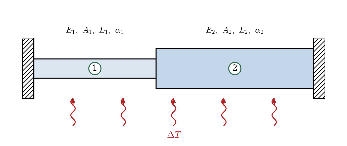
The same walls, but now two rods of different materials and cross sections joined in series between them, heated by \(\Delta T\).
Figure 8.11.6: Two rods in series between rigid walls.
Figure 8.11.7: Free body diagrams of the two rods and the junction.
Equilibrium of the two rods and the junction in Figure 8.11.7 passes the same normal force through both rods, since nothing is applied at the junction. Each rod may change length, but the walls have not moved, so the elongations must sum to zero. That compatibility condition decides the problem,
with the numerator collecting how much the assembly wants to expand and the denominator collecting how easily it gives way. Two rods of the same material reproduce Example 1, and a very compliant second rod, either long or thin or soft, drives \(N\) towards zero because it absorbs the expansion of the first. That is the principle behind an expansion loop.
Example 3: A rigid beam held by a rod
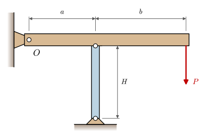
A rigid beam is hinged to a wall at \(O\) and carries a load \(P\) at its free end. A rod of a Hookean material, with cross-sectional area \(A\) and length \(H\), holds it up at the distance \(a\) from the hinge, as in Figure 8.11.8. Determine the stress in the rod and the deflection \(\Delta\) under the load.
Figure 8.11.8: A rigid beam hinged at \(O\), held up by a rod of length \(H\) and loaded by \(P\) at its end.
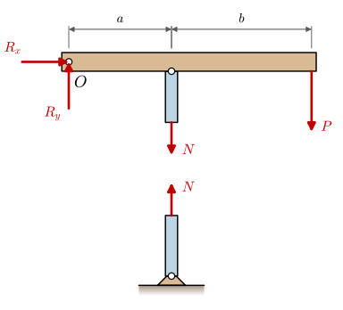
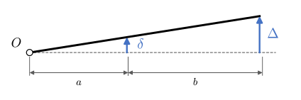
We cut the rod and set the normal force \(N\) positive out of the cut face, so that a positive \(N\) is tension. The deformation is drawn the same way, in the direction we take as positive: the rod lengthens by \(\delta\), and the rigid beam turns about \(O\) so that its end rises by \(\Delta\).
(a) The beam and the rod cut apart, with \(N\) out of both cut faces.
(b) The beam turned about \(O\), with \(\delta\) at the rod and \(\Delta\) at the load.
Figure 8.11.9: The free body diagram and the deformation of Example 3.
The three relations follow from Figure 8.11.9. Moments about \(O\) on the beam in Figure 8.11.9 (a) eliminate the hinge reactions, and the stress follows from the normal force. The strain of the rod is its elongation over its length, and since the beam is rigid it turns as a straight line about \(O\), so the similar triangles of Figure 8.11.9 (b) tie \(\delta\) to \(\Delta\). Hooke’s law closes the system,
which is five equations in the five unknowns \(N\), \(\sigma\), \(\varepsilon\), \(\delta\) and \(\Delta\).
N, sigma, eps, delta, Delta = sp.symbols('N sigma varepsilon delta Delta', real=True)P, a, b, H, E, A = sp.symbols('P a b H E A', positive=True)eqs = [sp.Eq((a + b)*P + a*N, 0), # moments about the hinge O sp.Eq(sigma, N/A), sp.Eq(eps, delta/H), sp.Eq(delta/a, Delta/(a + b)), # the rigid beam turns about O sp.Eq(sigma, E*eps)]sol = sp.solve(eqs, [N, sigma, eps, delta, Delta], dict=True)[0]sol = {k: sp.factor(v) for k, v in sol.items()}sol | la
\[ \begin{aligned}
\Delta &= - \dfrac{H P \left(a + b\right)^{2}}{A E a^{2}} \\[9.0pt]
N &= - \dfrac{P \left(a + b\right)}{a} \\[9.0pt]
\delta &= - \dfrac{H P \left(a + b\right)}{A E a} \\[9.0pt]
\sigma &= - \dfrac{P \left(a + b\right)}{A a} \\[9.0pt]
\varepsilon &= - \dfrac{P \left(a + b\right)}{A E a}
\end{aligned} \]
All five come out negative. The rod is in compression and shortens, so the beam turns downward and the load sinks by
The signs follow from setting \(N\) and \(\delta\) positive at the start, and they are what we expect: the load pushes the beam down onto the rod. The compressive force is larger than the load, \(|N| = P(a + b)/a\), because the rod sits closer to the hinge than the load does. The same lever ratio appears squared in the deflection, once through the force in the rod and once through the similar triangles that carry the shortening of the rod out to the load. Seen from the load, the structure is a spring of stiffness \(EA/H\) reduced by the square of the lever ratio. A rod that is long and slender compared with its cross section would also have to be checked for buckling, since it carries a compressive load.
Example 4: Stresses from a misfit
Stresses can arise in a structure with no load on it at all. Example 1 found them from a temperature change, and they arise just as well when parts that do not quite fit are forced together during assembly. Such stresses are called residual stresses, or eigenstresses.
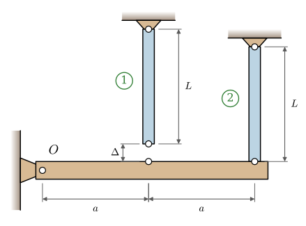
The rigid beam of Example 3 is now to be hung from two rods of a Hookean material, both of length \(L\) and cross-sectional area \(A\), attached at \(a\) and \(2a\) from the hinge \(O\). Rod 1 is too short by \(\Delta\), as in Figure 8.11.10, and has to be stretched to reach its pin on the beam. Determine the stresses in the rods once the beam is assembled.
Figure 8.11.10: Rod 1 ends \(\Delta\) short of its pin on the beam. Both rods have the length \(L\) and the area \(A\).
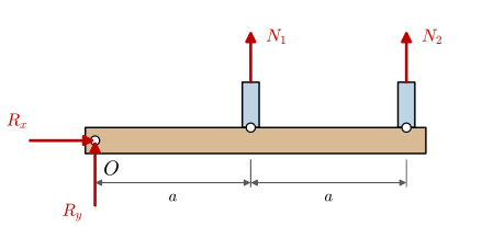
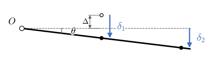
As before, both normal forces are set positive out of the cut faces, so that a positive \(N_i\) is tension, and the deformation is drawn the way we take as positive: both rods lengthen, and the beam turns clockwise by the small angle \(\theta\).
(a) The beam with both rods cut, \(N_1\) and \(N_2\) out of the cut faces.
(b) The assembled beam turned by \(\theta\) about \(O\). The end of rod 1 starts \(\Delta\) above the beam.
Figure 8.11.11: The free body diagram and the deformation of Example 4.
Moments about \(O\) on the beam in Figure 8.11.11 (a) give the only equilibrium relation that does not bring in the hinge reactions. The deformation relations come from Figure 8.11.11 (b). Rod 2 is pinned to the beam from the start, so the beam point under it sinks by \(\delta_2\). Rod 1 starts \(\Delta\) above its pin and reaches it by stretching \(\delta_1\), so the beam point under it sinks by \(\delta_1 - \Delta\). The beam is rigid, and both points lie on a straight line turned by \(\theta\) about \(O\),
Rod 1 has to be stretched to reach the beam, and in pulling the beam up it turns the beam anticlockwise, \(\theta = -\Delta/(5a)\), which pushes the beam up into rod 2. Of the misfit, \(4\Delta/5\) is taken up by stretching rod 1 and the remaining \(\Delta/5\) by the beam turning up to meet it. Rod 2, twice as far from the hinge, carries half the force of rod 1, so that their moments about \(O\) cancel.
The stresses depend on the misfit strain \(\Delta/L\) and the modulus, not on the area. A misfit of one millimetre in a one-metre steel rod gives \(E\Delta/L = 210~\text{GPa} \cdot 10^{-3} = 210~\text{MPa}\) and so \(\sigma_1 = 168~\text{MPa}\), a large stress with no load on the structure. Such stresses add to whatever the service loads produce, which is why tolerances matter in statically indeterminate assemblies. A statically determinate structure, like the beam held by one rod in Example 3, takes up a misfit by moving and carries no stress from it.
Where the diagram comes from
The English name used here is not standard. In Swedish teaching the figure is den gyllene kvadraten, and students who have met it elsewhere will recognise the four corners under that name, although its origin is hard to pin down: Swedish discussions of it attribute the term to textbook authors without naming one.
The diagram itself is older and more general than solid mechanics. Tonti [1] observed that the same square recurs throughout physics, with a configuration variable and a source variable joined by a chain of operators and a constitutive law across the middle, and he used it to classify a large number of field theories. The 1972 paper is hard to obtain; the construction is given book length treatment in [2]. What we have drawn for a bar is one cell of that classification.
Under Tonti’s name the diagram is standard in finite element teaching. Felippa [3] presents the governing equations of exactly our bar as a strong-form Tonti diagram, with unknown quantities in boxes of one colour and given data in another, and the field equations and boundary conditions drawn as the lines between them. He also uses a discrete version for what he calls mechanics-of-materials elements, which is the same square with matrices in place of derivatives. That is the version we meet in Chapter 8.14, where \(\bm A\), \(\bm S^e\) and \(\bm A^\mathsf{T}\) occupy the three sides. The three-relation grouping appears without the square in Ottosen and Petersson [4], who organise the entire finite element method around it.
What survives every renaming is the asymmetry between the three sides. Equilibrium and kinematics are statements about the world that hold whatever the bar is made of, and only the middle link changes when the material does. Replacing Hooke’s law by a plastic or a viscoelastic model redraws one side and leaves the other three untouched, which is why a single finite element code can handle all of them.
The Golden Quad and the continuum
Nothing in Figure 8.11.1 is restricted to one dimension. The four corners and three arrows are the same in the continuum, with each scalar replaced by its tensor counterpart, as we set out at the start of the chapter. A one-dimensional problem allows us to write the relations as scalar equations and solve them algebraically; a general problem forces the same relations into partial differential form and we solve them with the finite element method. The bookkeeping changes, the structure does not.
What we gain from the picture is a habit. Faced with an unfamiliar problem, ask which of the three relations are missing and write them down. A problem that statics alone cannot solve, meaning a statically indeterminate one, is always a problem in which the deformation relation carries information that equilibrium does not, and the missing equation is a statement about compatibility of displacements. Both examples above were of exactly this kind, and both were solved the moment the geometric condition was written down alongside the equilibrium equations.
The next chapter takes the same three relations and, instead of applying them to a finite bar, applies them to an infinitesimal slice. The result is the differential equation the bar formula 8.11.5 is a special solution of.
References
[1]
Tonti E. On the mathematical structure of a large class of physical theories. Atti Della Accademia Nazionale Dei Lincei, Classe Di Scienze Fisiche, Matematiche e Naturali, Rendiconti 1972;52:48–56.
[2]
Tonti E. The mathematical structure of classical and relativistic physics: A general classification diagram. New York: Birkhäuser; 2013.