The workflow

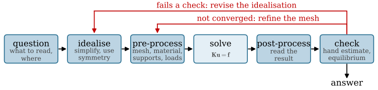
An analysis starts from a question, and the question decides the model. Will the A-arm of an RC car yield when the car lands a jump? How much does the chassis twist when one wheel hits a kerb? The first asks for the largest stress at one place, the second for the stiffness of the whole part, and the two call for different models of the same car. The question also names the result we will read at the end, a peak stress in a fillet or an angle of twist, and that result is what the mesh must resolve and what the checks must confirm. Writing the question down, with the quantity that answers it, is the first step.

The second step is idealisation: replacing the real part by a simpler model that keeps what governs the result and drops the rest. A CAD model carries lettering, small chamfers, threads and cosmetic fillets far from the region of interest, and they are removed, since each needs elements and none changes the answer. A bolted joint becomes a beam element or a rigid connection between the holes. Symmetry halves the model, or quarters it. A thin-walled part becomes a surface and a slender member a line, which is the step from the continuum to the theories of shells and beams that Chapter 8.16 made for bending. Every idealisation changes the result somewhere, and it is acceptable when it changes nothing near the place the question is about. We should be able to defend each one, since a model is only as good as its worst idealisation.

The remaining steps follow the order in which a program works. Pre-processing turns the idealised geometry into a numerical model. The geometry is divided into elements, the material model and its data are assigned to each part, supports and loads are attached as boundary conditions, and where parts touch each other contacts are defined. Solving forms the system of equations and solves it. The computer does this on its own, and although it may take hours, it is the step that needs the least of our time. Post-processing is reading the results, checking them, and drawing the conclusion that answers the question we started from. The sections below follow these steps, and Figure 8.20.1 draws them. The check at the end can send us back: to the mesh when the result has not converged, and to the idealisation when it fails a check.

Elements and the mesh

The method divides the part into a finite number of simple pieces, the elements. Inside each element the displacement is described by a simple function, usually a polynomial, fixed by its values at a small number of points. A node is such a point: a point where the unknown displacements are computed. Each unknown displacement or rotation at a node is a degree of freedom, and the whole collection of elements and nodes is the mesh. Producing it, mostly automatically from the CAD geometry, is called meshing.

The two-node rod of the rod equation chapter is the simplest element there is: two nodes, one degree of freedom at each, and the element stiffness matrix 8.12.8 that ties the two nodal forces to the two displacements. A solid part is meshed and assembled in the same way, from many more elements with more degrees of freedom each. Every element adds its stiffness matrix to the rows and columns of its own degrees of freedom, and the result is the global system

\[ \bm K\bm u = \bm f \tag{8.20.1}\]

with \(\bm K\) the global stiffness matrix, \(\bm u\) the vector of all nodal displacements and rotations and \(\bm f\) the vector of nodal forces. A model of a car part easily has a million degrees of freedom, but the system has the same structure as the chain of rods we assembled by hand. Once \(\bm u\) is known, the program differentiates the displacement inside each element to get the strains, 8.7.3, and turns them into stresses with Hooke’s law, 8.9.7. The displacements are the primary result. The stresses come from their derivatives, and on a given mesh they are less accurate than the displacements they come from.

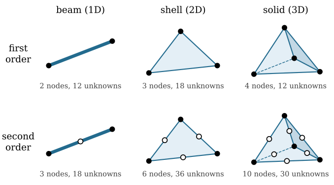
Elements come in three families, named after the dimension of the geometry they describe. A beam element (1D) is a line between two nodes for a member much longer than its cross section, a tube in a frame or a bolt. Each node has six degrees of freedom in space, three translations and three rotations, so a beam element brings twelve unknowns, and the cross section enters as properties such as \(A\), \(I\) and \(J\) that the bending and torsion theories of the earlier chapters use. A shell element (2D) is a triangle or a quadrilateral on the mid-surface of a thin-walled part, a sheet-metal bracket or an injection-moulded cover. Its nodes also have six degrees of freedom, and the wall thickness is a property, not part of the geometry. A solid element (3D) is a tetrahedron or a hexahedron that fills a volume and fits any shape. Its nodes have only the three translations.

Each family comes in a first-order and a second-order version. A first-order element interpolates the displacement linearly between its corner nodes, so the strain and the stress are constant, or nearly so, inside it. A second-order element adds a node on each edge, Figure 8.20.2, interpolates quadratically and lets the stress vary linearly across the element. A four-node tetrahedron has \(12\) degrees of freedom and a ten-node tetrahedron \(30\). The second-order element costs more per element and far less per unit of accuracy. The four-node tetrahedron is also too stiff in bending: a beam meshed with a handful of them deflects much less than it should. Automatic meshers fill a solid with tetrahedra, as they would for any printed or cast part, and those tetrahedra should be of second order.

The stress in a bent wall varies linearly through the thickness, from tension at one face to compression at the other, 8.16.10. One layer of first-order solid elements has a single constant stress across the wall and cannot represent this at all, and even second-order elements need several layers to reach the stress at the faces. The rule of thumb is at least three solid elements through any thickness that carries bending. A thin wall that would need very small solid elements to meet that rule is the case for shell elements, which carry the linear variation through the thickness in their formulation.

Boundary conditions

An unsupported part has a singular stiffness matrix for the same reason the rod element had: nothing stops it from moving as a rigid body, and a rigid motion changes no force. Boundary conditions remove that freedom and bring in the loads. The accounting rule of Known and unknown holds at every degree of freedom: either the displacement is prescribed and the force is an unknown reaction, or the force is prescribed, possibly as zero, and the displacement is unknown.

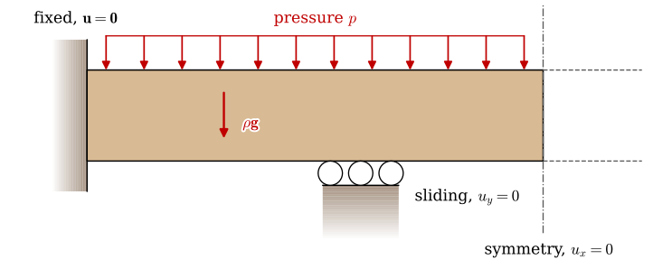
The two kinds of condition are those of the rod’s boundary value problem, 8.12.5, carried over to a solid. A Dirichlet boundary condition prescribes the primary variable, a displacement or a rotation, on part of the boundary. A fixed support sets every displacement on a face to zero. A sliding support sets only the displacement normal to a face to zero and lets the face slide in its plane. A symmetry condition is a sliding support on a plane of symmetry: material on the plane cannot cross it, since its mirror image would have to cross it the other way, but it may move along the plane. A Neumann boundary condition prescribes the gradient of the primary variable, which through Hooke’s law is a stress and therefore a force: a pressure on a face, a force spread over an edge or a face, or gravity, which acts on every element as a body load. Dirichlet conditions remove unknowns from 8.20.1, the way 8.12.10 struck out the prescribed rows of the chain. Neumann conditions enter the load vector \(\bm f\) and leave the unknowns as they were. A free surface is also a Neumann condition, with zero traction, and every model has it on every face we leave alone. Figure 8.20.3 puts the common conditions on one part: half of a beam, built into a wall at its left end, resting on a sliding support, cut at its plane of symmetry, and loaded by a pressure on its top face and by its own weight.

Both kinds are idealisations. No real support is rigid. A bolted flange bends, a clamp lets the part slip a little and a bolt hole ovalises. A fixed face also forbids the Poisson contraction of the material on it, which a real support permits, and the mismatch produces a stress at the edge of the fixed face that the real part does not have. A point force is worse. A finite force on one node acts on zero area, and the stress under it grows without limit as the mesh is refined, while a real force always spreads over a contact patch of some size. Supports and loads therefore belong on areas of realistic size, and the stresses right next to them are artefacts of how the model is held and loaded, a point we return to in Reading the results.

The linear assumptions

A standard static analysis forms \(\bm K\) once, in the undeformed geometry, and solves 8.20.1 once. That is a linear analysis, and it rests on three assumptions.

The first is that the displacements are small. Equilibrium is then written on the undeformed shape, the stiffness does not change as the part deforms, and doubling the load doubles every displacement and every stress. The assumption breaks when the deformation changes the way the load is carried: a thin plate that bulges under pressure and starts to carry it as a membrane, a column near its buckling load, Chapter 8.18, or a snap-fit that bends far. Such cases need a geometrically nonlinear analysis that updates the geometry as the load grows. Contact is nonlinear for the same reason, since the area in contact changes with the load.

The second is that the material is linear elastic, Hooke’s law with constant \(E\) and \(\nu\), so that the part returns to its original shape when the load is removed. The assumption breaks when the material yields. For most plastics, printed ones included, it holds only at small strains, since their stress-strain curves bend away from the initial line early, Chapter 8.6.

The third is that the loads are static, applied slowly enough that inertia plays no part. The assumption breaks under impact and vibration, when the car lands a jump or hits a wall. Such loads need a dynamic analysis, implicit with large time steps for vibration, or explicit for crash and impact, with time steps short enough that a stress wave crosses no element in one step.

The second assumption breaks without warning. A linear model does not know that the material has a yield strength, and it reports whatever stress Hooke’s law gives, \(600~\text{MPa}\) in a steel that yields at \(355~\text{MPa}\) or \(90~\text{MPa}\) in a printed PLA part that breaks at \(50~\text{MPa}\). That is linear analysis above yield, and the number does not mean that the real stress is that high. It means that linear theory no longer holds at that point. The real material yields, the stress in the yielded zone stays near the yield strength, and the load moves to the material around it. A finer mesh changes nothing, since it solves the same linear model more accurately and makes the meaningless number more precise. A computed stress above yield is a statement about the validity of the model. A small yielded zone at a stress concentration in a ductile part under a static load is often harmless, as Chapter 8.19 discussed, while a whole cross section above yield means that the part has failed. What the material does beyond yield is the subject of plasticity, Chapter 8.17, and how a solver handles it is the subject of its section Computational plasticity.

Stress concentration or singularity

By 8.19.4 of Sharp notches, the peak stress at the tip of an elliptical hole is \(\sigma\left(1 + 2\sqrt{a/\rho}\right)\), finite for every tip radius \(\rho > 0\) and unbounded as \(\rho \to 0\). A finite element model inherits both cases. Where the part has a radius and the model contains it, the computed peak converges to \(K_t\sigma_{\text{nom}}\) as the mesh is refined. That stress is high but finite, and it is physical: the real part carries it, and a fatigue crack will start there.

A sharp re-entrant corner, one where the boundary turns into the material so that the material occupies more than half the plane around the corner point, has \(\rho = 0\). The inside corner of an L-bracket and the foot of a shoulder without a fillet are examples. Close to such a corner the elasticity solution has no finite peak. Williams found the form of the field in 1952 [1]: at a distance \(\rho\) from the corner point the stresses grow as

\[ \sigma \propto \rho^{\lambda - 1} \tag{8.20.2}\]

with an exponent \(\lambda\) between \(\tfrac{1}{2}\) and \(1\) that depends only on the interior angle \(\alpha\) of the corner. For the strongest of these fields, the one that dominates closest to the corner, \(\lambda\) is the smallest positive root of

\[ \sin\lambda\alpha = -\lambda\sin\alpha \tag{8.20.3}\]

which gives \(\lambda = \tfrac{1}{2}\) for a crack, \(\alpha = 2\pi\), and \(\lambda = 1\), no singularity, for a straight edge, \(\alpha = \pi\). A right-angled re-entrant corner has \(\alpha = 3\pi/2\), so that \(\sin(3\pi\lambda/2) = \lambda\), \(\lambda = 0.544\), and the stress grows as \(\rho^{-0.456}\). A point where the stress of the continuum model is infinite is a singularity. A mesh cannot represent an infinite stress, so the elements at the corner report a finite value, roughly the average of 8.20.2 over their own size. The smaller the elements, the larger that average. Every refinement gives a higher peak, and no mesh gives the answer, because the model has none.

A stress concentration is physical, and a singularity is numerical. Sharp corners cause both. No real part has a corner of zero radius: a milled inside corner has the radius of the cutter and a printed one is rounded by the width of the extruded line. That radius is small, so the real peak is high and the real part is weakened. The model without the radius reports a number that depends on the mesh and not on the part.

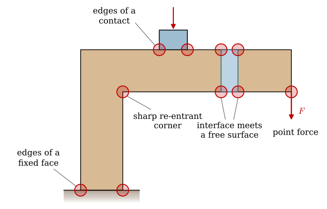
Singularities appear wherever the model contains something infinitely sharp or infinitely stiff that the real part does not. Sharp re-entrant corners and crack tips are the geometric sources. The boundary conditions add their own: a fixed support at the edges of the fixed face, a point force at the loaded node and a rigid connection at the nodes it ties together. A contact with a sharp edge, a washer on a plate or a flat punch on a surface, gives a singularity at the edge of the contact zone, and so does the line where an interface between two bonded materials of different stiffness meets a free surface. Figure 8.20.4 marks all of them on one bracket.

There are two remedies. When the stress at the corner is what we need, the model must contain the real radius, meshed finely enough for the peak to converge, and if the radius is not known, choosing a small, conservative one is a design decision to be written down. When the corner lies away from the question, the singularity can stay in the model and the stress is read some distance from it, several elements away, where the solution converges as it does anywhere else. Refining the mesh at the singular point is not a remedy. The better remedy is in the design: a fillet of generous radius lowers the physical peak and removes the singularity at the same time.

Mesh convergence

Every finite element result carries a discretisation error, the difference between the solution on the mesh and the solution of the continuum model the mesh approximates. We cannot compute that error, since the exact solution is unknown, but we can watch it shrink. A mesh convergence study solves the same model on a sequence of finer meshes, refined where the result of interest lives, and records that result each time. When it stops changing appreciably, by less than a few percent between two successive meshes, the mesh is fine enough for that result. A result that keeps changing has not converged, and a peak that keeps growing at one point is a singularity. Convergence belongs to a result and not to a mesh. A mesh that has converged the deflection of a bracket can be far too coarse for the peak stress in its fillet, since stresses are derivatives of the displacements and converge more slowly.

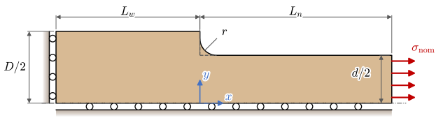
We now carry out such a study for both cases of the previous section. The model is the stepped flat bar of Chapter 8.19 in tension, Figure 8.20.5. The bar is \(t = 1~\text{mm}\) thick and narrows from \(D = 30~\text{mm}\) to \(d = 20~\text{mm}\), and the shoulder has either a fillet of radius \(r = 2~\text{mm}\) or a sharp corner, \(r = 0\). The bar is symmetric about its centre line, so we model the upper half and replace the lower half by the symmetry condition \(u_y = 0\) on \(y = 0\). The wide end slides along a wall, \(u_x = 0\) at \(x = -L_w\), and the narrow end carries the uniform traction \(\sigma_{\text{nom}} = F/(dt) = 100~\text{MPa}\). Uniform tension satisfies both supports exactly, so neither is singular and the shoulder is the only sharp feature. With \(L_w = 30~\text{mm}\) and \(L_n = 40~\text{mm}\) both ends lie more than a section width from the shoulder, as Saint-Venant’s principle of Section 8.3.9 asks. The steel has \(E = 210~\text{GPa}\) and \(\nu = 0.3\), although neither affects the stresses, which in this model are set by the geometry and the load alone.

For the filleted shoulder the chart gives the answer in advance. With \(h = (D - d)/2 = 5~\text{mm}\), the bar has \(h/r = 2.5\) and \(2h/D = 1/3\), inside the range of the fit 8.19.6, and \(K_t\sigma_{\text{nom}}\) is the peak the model should converge to. RoyMech tabulates \(2.24\) for this geometry¹. For the sharp corner the previous section gives no such value, since the stress there grows without bound, 8.20.2.

D, d, r_fillet = 30.0, 20.0, 2.0                # mm, the wide and the narrow width, the fillet radius
h_step = (D - d)/2                              # the height of the step on each side
q, x = h_step/r_fillet, 2*h_step/D              # h/r and 2h/D of @eq-kt-fit
# the coefficients c_ij of @eq-kt-fit for the stepped flat bar in tension, the set for h/r > 2
c = [(1.042, 0.982, -0.036), (-0.074, -0.156, -0.010), (-3.418, 1.220, -0.005), (3.450, -2.046, 0.051)]
K_t = sum((c1 + c2*np.sqrt(q) + c3*q)*x**i for i, (c1, c2, c3) in enumerate(c))

ltx(r"K_t =", K_t, precision=3)

We solve the model with three-node triangles, the simplest element for a plane problem. Each triangle deforms with one constant strain and therefore carries one constant stress, so a stress plot of the model is a patchwork with one flat colour per triangle. The code below meshes the bar, assembles \(\bm K\bm u = \bm f\), solves it and computes the stresses of every element, and the later sections of this chapter reuse it. The result we follow through the refinements is the largest first principal stress of any element, divided by the nominal stress,

\[ K_h = \frac{\max_e \sigma_1^e}{\sigma_{\text{nom}}} \tag{8.20.4}\]

which for the filleted shoulder should approach \(K_t\). In this plane stress model \(\sigma_1^e\) is the larger in-plane principal stress of 8.7.12, \(\sigma_\text{I}\) in the notation of Principal stresses in three dimensions. The out-of-plane principal stress is zero, so \(\sigma_\text{I}\) is also the ordered \(\sigma_1\) wherever it is positive, as it is at the shoulder of a bar in tension. At the free surface of the fillet the stress is uniaxial, along the surface, so there \(\sigma_1\) and the von Mises stress coincide.

The meshes are graded. The element size is \(h\) within \(3~\text{mm}\) of the foot of the shoulder and grows away from it, up to \(4~\text{mm}\) at the ends, and Shewchuk’s mesh generator Triangle² fills the outline with triangles whose angles are all at least \(30^\circ\). Both geometries get the same sizes, and \(h\) is halved ten times, from \(2~\text{mm}\), the fillet radius, to \(2/1024~\text{mm}\).

B, b = D/2, d/2                      # the half widths, since we model the upper half
L_w, L_n = 30.0, 40.0                # mm, the lengths of the wide and the narrow part
E, nu, t = 210e3, 0.3, 1.0           # MPa and mm, so that forces come out in N
sigma_nom = 100.0                    # MPa, the traction on the narrow end


def outline(r):
    """The boundary of the half bar, walked anticlockwise, as lines and, for r > 0, one arc."""
    if r == 0:
        shoulder = [('line', (L_n, b), (0, b)), ('line', (0, b), (0, B))]
    else:
        # the fillet's centre lies outside the material, at (r, b + r)
        shoulder = [('line', (L_n, b), (r, b)), ('arc', (r, b + r), r, 1.5*np.pi, np.pi),
                    ('line', (0, b + r), (0, B))]
    return ([('line', (-L_w, 0), (L_n, 0)), ('line', (L_n, 0), (L_n, b))] + shoulder
            + [('line', (0, B), (-L_w, B)), ('line', (-L_w, B), (-L_w, 0))])


def point(piece, s):
    """The point a fraction s of the way along one piece of the outline."""
    if piece[0] == 'line':
        p0, p1 = np.array(piece[1]), np.array(piece[2])
        return p0 + s*(p1 - p0)
    _, centre, R, a0, a1 = piece
    a = a0 + s*(a1 - a0)
    return np.array(centre) + R*np.array([np.cos(a), np.sin(a)])


def size(p, h):
    """The element size wanted at p: h near the foot of the shoulder, coarser away from it."""
    return min(4.0, h + 0.3*max(0.0, np.hypot(p[0], p[1] - b) - 3.0))


def triangulate(pieces, size_at):
    """Nodes and three-node triangles inside the outline, sized by the function size_at."""
    pts = []
    for piece in pieces:
        s = np.linspace(0, 1, 2001)
        xy = np.array([point(piece, si) for si in s])
        density = 1/np.array([size_at(p) for p in xy])                # elements per mm
        dl = np.linalg.norm(np.diff(xy, axis=0), axis=1)
        count = np.r_[0, np.cumsum(dl*(density[:-1] + density[1:])/2)]  # elements so far
        n = max(1, int(np.ceil(count[-1])))
        # one boundary node at each whole element count along the piece
        pts += [point(piece, si) for si in np.interp(np.linspace(0, count[-1], n + 1)[:-1], count, s)]
    m = len(pts)
    segments = np.c_[np.arange(m), (np.arange(m) + 1) % m]
    # p: keep the outline, q30: no angle below 30 degrees, a8: no triangle above 8 mm^2
    out = triangle.triangulate({'vertices': np.array(pts), 'segments': segments}, 'pq30a8')
    return out['vertices'], out['triangles']


def mesh(r, h):
    """Nodes and three-node triangles of the half bar with fillet radius r and size h."""
    return triangulate(outline(r), lambda p: size(p, h))

C = E/(1 - nu**2)*np.array([[1, nu, 0],
                            [nu, 1, 0],
                            [0, 0, (1 - nu)/2]])         # Hooke's law in plane stress


def stiffness(X, T):
    """The global stiffness matrix, with each element's B matrix and degrees of freedom."""
    n_dof = 2*len(X)
    dofs = np.stack([2*T, 2*T + 1], axis=2).reshape(-1, 6)   # u_x, u_y of the element's nodes 1, 2, 3
    Bs, rows, cols, vals = [], [], [], []
    for el, dof in zip(T, dofs):
        x, y = X[el, 0], X[el, 1]
        A = ((x[1] - x[0])*(y[2] - y[0]) - (x[2] - x[0])*(y[1] - y[0]))/2
        b_i = np.array([y[1] - y[2], y[2] - y[0], y[0] - y[1]])
        c_i = np.array([x[2] - x[1], x[0] - x[2], x[1] - x[0]])
        Be = np.zeros((3, 6))
        Be[0, 0::2], Be[1, 1::2] = b_i, c_i
        Be[2, 0::2], Be[2, 1::2] = c_i, b_i
        Be /= 2*A                                                  # the constant strain of the triangle
        ke = t*A*Be.T @ C @ Be                                     # the element stiffness
        Bs.append(Be)
        # each entry of ke lands in the global row and column of its two degrees of freedom
        rows.append(np.repeat(dof, 6)); cols.append(np.tile(dof, 6)); vals.append(ke.ravel())
    K = sps.csr_matrix((np.concatenate(vals), (np.concatenate(rows), np.concatenate(cols))),
                       shape=(n_dof, n_dof))                       # duplicates are summed
    return K, np.array(Bs), dofs


def end_load(X, x_end):
    """Neumann: each element edge on the end x = x_end carries sigma_nom t l, half to each node."""
    f = np.zeros(2*len(X))
    end = np.flatnonzero(np.isclose(X[:, 0], x_end))
    end = end[np.argsort(X[end, 1])]
    for i, j in zip(end[:-1], end[1:]):
        f[[2*i, 2*j]] += sigma_nom*t*(X[j, 1] - X[i, 1])/2
    return f


def fe_solve(X, T, p, f):
    """Solve with u = 0 on the degrees of freedom p; the stresses of every element."""
    K, Bs, dofs = stiffness(X, T)
    free = np.setdiff1d(np.arange(2*len(X)), p)
    u = np.zeros(2*len(X))
    u[free] = spla.spsolve(K[free][:, free].tocsc(), f[free])      # with u = 0 on the supported dofs
    sig = np.einsum('ij,ejk,ek->ei', C, Bs, u[dofs])               # sigma_x, sigma_y, tau_xy per element
    s1 = (sig[:, 0] + sig[:, 1])/2 + np.hypot((sig[:, 0] - sig[:, 1])/2, sig[:, 2])
    return dict(X=X, T=T, sig=sig, s1=s1, K=s1.max()/sigma_nom, n_el=len(T), p=p, R=(K @ u - f)[p])


def solve(r, h):
    """Mesh, load, support and solve the half bar with fillet radius r and element size h."""
    X, T = mesh(r, h)
    # Dirichlet: u_x = 0 where the wide end slides on the wall, u_y = 0 on the symmetry line
    p = np.r_[2*np.flatnonzero(np.isclose(X[:, 0], -L_w)), 2*np.flatnonzero(np.isclose(X[:, 1], 0)) + 1]
    return fe_solve(X, T, p, end_load(X, L_n))


h_list = 2.0/2**np.arange(11)                                      # mm, 2 down to 2/1024
study = {r: [solve(r, h) for h in h_list] for r in (2.0, 0.0)}

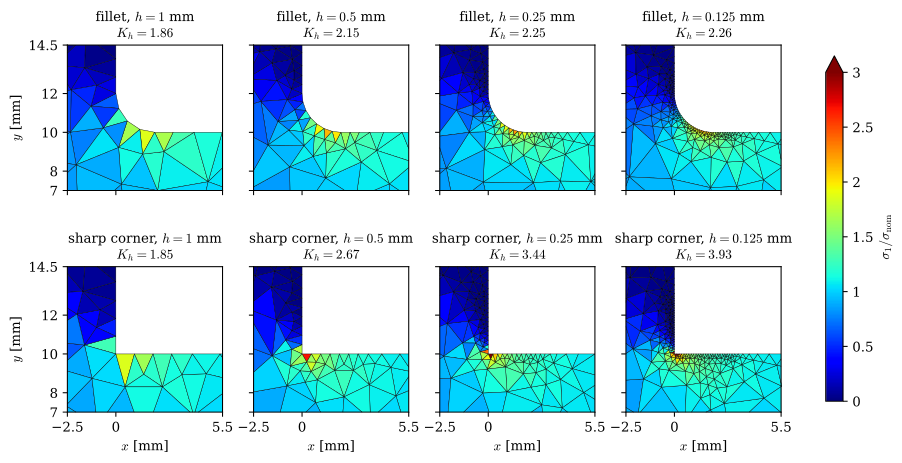
Figure 8.20.6 shows what the refinement does near the shoulder. From left to right the element size is halved three times, from \(h = 1~\text{mm}\) to \(0.125~\text{mm}\), and each panel shows the mesh in the same small window with every triangle coloured by its first principal stress, on one colour scale for all eight panels.

With the fillet, in the top row, the first mesh puts only three elements along the curve, and its peak is too low. The next meshes follow the curve more closely, and the coloured band along the fillet keeps its size and its shape from one panel to the next. The finer triangles only draw the same field more sharply, and the peak settles close to \(K_t\).

With the sharp corner, in the bottom row, nothing settles. The hot zone shrinks into the corner as the triangles shrink, and the triangle that touches the corner reports a higher stress on every mesh. Away from the corner the two rows look alike, since a millimetre from the shoulder the bar does not notice whether the corner is rounded. On the coarsest mesh the two peaks are even the same, \(1.86\) against \(1.85\): one coarse model cannot tell a fillet from a singularity, and only the refinement shows which of the two we have.

ks = [1, 2, 3, 4]                                              # h = 1, 0.5, 0.25, 0.125 mm
top = 3.0                                                      # one scale; the corner saturates
fig, axes = plt.subplots(2, 4, figsize=(12, 5.5), sharex=True, sharey=True)
for row, (r, name) in enumerate(((2.0, 'fillet'), (0.0, 'sharp corner'))):
    for col, k in enumerate(ks):
        ax, s = axes[row, col], study[r][k]
        pc = ax.tripcolor(s['X'][:, 0], s['X'][:, 1], s['T'], facecolors=s['s1']/sigma_nom,
                          cmap='jet', vmin=0, vmax=top, edgecolors='k', linewidth=0.3)
        ax.set_xlim(-2.5, 5.5)
        ax.set_ylim(7.0, 14.5)
        ax.set_aspect('equal')
        ax.set_title(f"{name}, $h = {h_list[k]:g}$ mm\n" + rf"$K_h = {s['K']:.2f}$", fontsize=10)
for ax in axes[1]:
    ax.set_xlabel('$x$ [mm]')
for ax in axes[:, 0]:
    ax.set_ylabel('$y$ [mm]')
fig.colorbar(pc, ax=axes, label=r'$\sigma_1/\sigma_{\mathrm{nom}}$', shrink=0.85, extend='max')
end_ticks(fig)
plt.show()

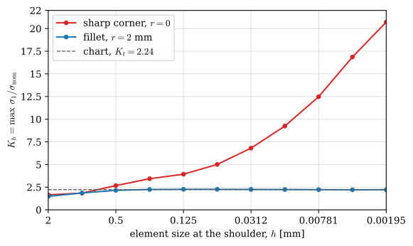
Figure 8.20.7 follows the peak 8.20.4 through all eleven meshes. The filleted shoulder levels off. Once the elements are smaller than about an eighth of the radius, \(h \le 0.25~\text{mm}\), the peak changes by less than one percent from one mesh to the next and stays between \(2.21\) and \(2.26\), within one and a half percent of the chart value \(K_t = 2.24\), a fit that itself scatters by several percent about the measurements behind it. The sharp corner does not level off. On the fine meshes every halving of the element size raises its peak by about a third, and on the finest, with \(h = 0.002~\text{mm}\), it has reached \(20.7\,\sigma_{\text{nom}}\), more than nine times the filleted value, with nothing in the curve to suggest a limit.

fig, ax = plt.subplots(figsize=(6.4, 3.8))
ax.plot(h_list, [s['K'] for s in study[0.0]], 'o-', color='C3', ms=4, label='sharp corner, $r = 0$')
ax.plot(h_list, [s['K'] for s in study[2.0]], 'o-', color='C0', ms=4, label='fillet, $r = 2$ mm')
ax.axhline(K_t, color='0.35', ls='--', lw=1, label=f'chart, $K_t = {K_t:.2f}$')
ax.set_xscale('log')
ax.set_xlim(h_list[0], h_list[-1])                       # coarse on the left, fine on the right
ax.set_xticks(h_list[::2], labels=[f'{v:.3g}' for v in h_list[::2]])
ax.minorticks_off()
ax.set_ylim(0, np.ceil(1.02*max(s['K'] for s in study[0.0])))
ax.set_xlabel('element size at the shoulder, $h$ [mm]')
ax.set_ylabel(r'$K_h = \max\,\sigma_1/\sigma_{\mathrm{nom}}$')
ax.grid(True, alpha=0.4)
ax.legend(loc='upper left')
end_ticks(fig)
plt.show()

The difference between the two curves lies in the continuum problem that the meshes approximate. With the fillet, the exact stress of the elastic bar is a smooth field with a largest value on the curved surface, \(K_t\sigma_{\text{nom}}\). A constant-stress triangle reports roughly the average of that field over its own area. Once the triangles are small compared with the radius, the field barely changes across a triangle at the surface, and the average there is close to the surface value. Halving the triangles again changes that average by little, and the sequence of peaks closes in on one number. That is what convergence means: the meshes approach the answer of the continuum model.

With the sharp corner the continuum model has no largest value to approach. The exact stress grows without bound towards the corner, 8.20.2, and the triangle at the corner averages that field over a smaller region, closer to the corner, on every mesh. Its value rises with each refinement and would go on rising on any finer mesh we could afford. The \(20.7\,\sigma_{\text{nom}}\) of the finest mesh says how small its elements are, not how the part is loaded. A real shoulder has a small radius, and its peak is the converged value for that radius.

The study gives a working rule. Refine where the result lives, at least three times, and follow that result. If it levels off, the mesh is fine enough for that result. If it keeps rising at one point, look there for a sharp corner, a point load or a rigid edge, and model what the real part has.

Reading the results

A program can plot any component of the stress tensor, and the first decision is which one answers the question. For a ductile metal the yield criterion of Chapter 8.7 applies, and the von Mises effective stress 8.7.22, compared with the yield strength, gives the factor of safety against yielding. It carries no sign, so it does not tell tension from compression. A brittle material, such as cast iron, glass or a ceramic, fails from cracks that open under tension, and the first principal stress \(\sigma_1\) compared with the tensile strength is the measure. A compressive peak matters in such a material only when it is large, since its compressive strength is several times its tensile strength. A part printed by fused deposition is brittle in one direction. The bond between two layers is much weaker than the extruded line, and a part pulled across its layers breaks along an interface with little warning, so for a printed part the first principal stress, or the normal stress in the build direction, is compared with the strength across the layers.

The stresses are computed inside each element, at its integration points, and in a first-order element they are constant or nearly so. Two elements that share a node give two different values there, since the stress of a displacement-based model jumps across element boundaries, and a plot of the element stresses is a patchwork, as in Figure 8.20.6. Most post-processors smooth it by averaging, at each node, the values of the elements around it, and plot the nodal or averaged stress. The averaged plot looks smoother but hides the jumps, and at a peak on a surface it reports a lower value, since it mixes the peak element with less loaded neighbours. The difference between the two is a free estimate of the discretisation error: where the element and the averaged peak differ by more than a few percent, the mesh is too coarse for that stress. The simplest averaging weights each element by its area. At node \(n\) the averaged stress components are

\[ \bar{\bm\sigma}_n = \frac{\sum_{e \ni n} A_e\,\bm\sigma^e}{\sum_{e \ni n} A_e} \tag{8.20.5}\]

where the sums run over the elements that share node \(n\), \(\bm\sigma^e = [\sigma_x, \sigma_y, \tau_{xy}]^\mathsf{T}\) is the constant stress of element \(e\) and \(A_e\) is its area. The first principal stress at the node follows from the averaged components by 8.7.12, and the plot interpolates it linearly inside each triangle. We apply this to every mesh of the filleted shoulder.

def nodal_s1(s):
    """The first principal stress at the nodes, from the averaged components of @eq-fea-nodal-average."""
    X, T = s['X'], s['T']
    x, y = X[T, 0], X[T, 1]
    A = ((x[:, 1] - x[:, 0])*(y[:, 2] - y[:, 0]) - (x[:, 2] - x[:, 0])*(y[:, 1] - y[:, 0]))/2
    num, den = np.zeros((len(X), 3)), np.zeros(len(X))
    for k in range(3):                     # every element hands its weighted stress to each of its nodes
        np.add.at(num, T[:, k], A[:, None]*s['sig'])
        np.add.at(den, T[:, k], A)
    sn = num/den[:, None]
    return (sn[:, 0] + sn[:, 1])/2 + np.hypot((sn[:, 0] - sn[:, 1])/2, sn[:, 2])


for s in study[2.0]:
    s['s1_nodal'] = nodal_s1(s)
    s['K_nodal'] = s['s1_nodal'].max()/sigma_nom

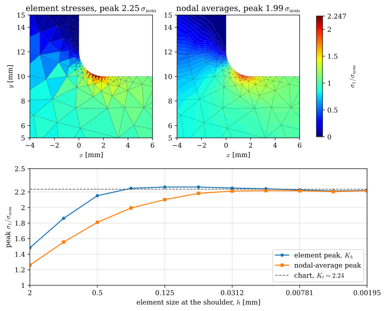
Figure 8.20.8 compares the two plots on the mesh with \(h = 0.25~\text{mm}\), the mesh on which the element peak had settled within one percent of its limit, and follows both peaks through the refinements.

k = 3                                                          # h = 0.25 mm
s = study[2.0][k]
top = s['s1'].max()/sigma_nom
fig = plt.figure(figsize=(9, 7.4))
grid = fig.add_gridspec(2, 2, height_ratios=[1.15, 1])
ax_e, ax_n = fig.add_subplot(grid[0, 0]), fig.add_subplot(grid[0, 1])
ax_c = fig.add_subplot(grid[1, :])
pc = ax_e.tripcolor(s['X'][:, 0], s['X'][:, 1], s['T'], facecolors=s['s1']/sigma_nom,
                    cmap='jet', vmin=0, vmax=top, edgecolors='k', linewidth=0.15)
# linear interpolation between the nodes, drawn as many narrow colour bands
ax_n.tricontourf(s['X'][:, 0], s['X'][:, 1], s['T'], s['s1_nodal']/sigma_nom,
                 levels=np.linspace(0, top, 61), cmap='jet', vmin=0, vmax=top)
ax_n.triplot(s['X'][:, 0], s['X'][:, 1], s['T'], color='k', lw=0.15)
for ax, title, K in ((ax_e, 'element stresses', s['K']), (ax_n, 'nodal averages', s['K_nodal'])):
    ax.set_xlim(-4, 6)
    ax.set_ylim(5, 15)
    ax.set_aspect('equal')
    ax.set_title(f"{title}, peak {K:.2f}" + r"$\,\sigma_{\mathrm{nom}}$")
    ax.set_xlabel('$x$ [mm]')
ax_e.set_ylabel('$y$ [mm]')
fig.colorbar(pc, ax=[ax_e, ax_n], label=r'$\sigma_1/\sigma_{\mathrm{nom}}$', shrink=0.9)

ax_c.plot(h_list, [s['K'] for s in study[2.0]], 'o-', color='C0', ms=4, label='element peak, $K_h$')
ax_c.plot(h_list, [s['K_nodal'] for s in study[2.0]], 's-', color='C1', ms=4, label='nodal-average peak')
ax_c.axhline(K_t, color='0.35', ls='--', lw=1, label=f'chart, $K_t = {K_t:.2f}$')
ax_c.set_xscale('log')
ax_c.set_xlim(h_list[0], h_list[-1])
ax_c.set_xticks(h_list[::2], labels=[f'{v:.3g}' for v in h_list[::2]])
ax_c.minorticks_off()
ax_c.set_ylim(1, 2.5)
ax_c.set_xlabel('element size at the shoulder, $h$ [mm]')
ax_c.set_ylabel(r'peak $\sigma_1/\sigma_{\mathrm{nom}}$')
ax_c.grid(True, alpha=0.4)
ax_c.legend(loc='lower right')
end_ticks(fig)
plt.show()

gap = [100*(s['K'] - s['K_nodal'])/s['K'] for s in study[2.0]]   # percent of the element peak
ltx(r"h = 0.25~\text{mm}:\quad K_h &=", study[2.0][3]['K'], r",\quad \max\bar\sigma_1/\sigma_{\text{nom}} =",
    study[2.0][3]['K_nodal'], r",\quad \text{difference} =", gap[3], r"~\%"
    r"\\ h = 2/1024~\text{mm}:\quad K_h &=", study[2.0][-1]['K'], r",\quad \max\bar\sigma_1/\sigma_{\text{nom}} =",
    study[2.0][-1]['K_nodal'], r",\quad \text{difference} =", gap[-1], r"~\%",
    aligned=True, precision=3)

On the mesh with \(h = 0.25~\text{mm}\) the averaged plot is smooth and looks finished, and its peak is \(11\) percent below the element peak, which is already within one percent of the chart. The averaging spreads the peak element over its less loaded neighbours, and the smooth plot gives no sign of it. As the elements shrink the two peaks approach each other, and on the finest mesh they differ by \(0.2\) percent. A difference of more than a few percent between the element and the averaged peak therefore says that the mesh is too coarse for that peak, and it is available on every mesh without a second solve.

The peak that a post-processor reports is the largest value anywhere in the model, and it is often in the wrong place. Next to a fixed face, a rigid connection or a node that carries a point load, the stress depends on how the model is held and loaded, and the singularities of Stress concentration or singularity put the largest numbers there. Saint-Venant’s principle of Section 8.3.9 tells us how far the effect reaches: the way a load is introduced changes the stress only within about one section depth of the place where it enters, and beyond that distance the stress depends on the resultant alone. We therefore read stresses at least a section depth from supports and load points. When the stress at a support is itself the question, the support has to be modelled as it is, with the bolt, its washer and the contact between them, or the pin in its hole.

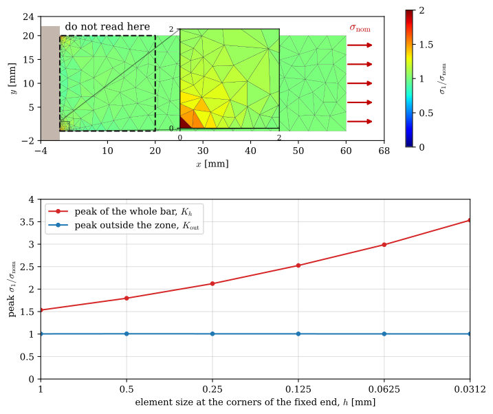
A bar fixed at one end shows the effect. The bar is \(L_f = 60~\text{mm}\) long, \(W_f = 20~\text{mm}\) wide and \(t = 1~\text{mm}\) thick, of the same steel as before, and carries the traction \(\sigma_{\text{nom}} = 100~\text{MPa}\) on its free end. Its other end is fixed, \(u_x = u_y = 0\) on \(x = 0\), the way a bar welded to a rigid wall is often modelled (Figure 8.20.9, top). The fixed end forbids the Poisson contraction of the material on it, which the rest of the bar undergoes, so the two corners of the fixed end are singular points of the kind listed in Stress concentration or singularity. Uniform tension, \(\sigma_x = \sigma_{\text{nom}}\) and nothing else, is the exact solution everywhere else once Saint-Venant’s principle has done its work. We mesh the bar with the triangles of the stepped bar, graded towards the two corners with the size \(h\) there, and follow two numbers through the refinements: the peak \(K_h\) of 8.20.4 over the whole bar, and the peak outside the zone within one width of the fixed end,

\[ K_{\text{out}} = \frac{1}{\sigma_{\text{nom}}}\max_{e:\,x_e \ge W_f}\sigma_1^e \tag{8.20.6}\]

where \(x_e\) is the \(x\) coordinate of the centroid of element \(e\).

L_f, W_f = 60.0, 20.0                       # mm, the length and the width of the fixed bar
bar = [('line', (0, 0), (L_f, 0)), ('line', (L_f, 0), (L_f, W_f)),
       ('line', (L_f, W_f), (0, W_f)), ('line', (0, W_f), (0, 0))]


def size_fixed(p, h):
    """The element size wanted at p: h at the two corners of the fixed end, coarser away from them."""
    return min(4.0, h + 0.3*max(0.0, min(np.hypot(p[0], p[1]), np.hypot(p[0], p[1] - W_f)) - 2.0))


def solve_fixed(h):
    X, T = triangulate(bar, lambda p: size_fixed(p, h))
    wall = np.flatnonzero(np.isclose(X[:, 0], 0))
    s = fe_solve(X, T, np.r_[2*wall, 2*wall + 1], end_load(X, L_f))    # u_x = u_y = 0 on x = 0
    s['K_out'] = s['s1'][X[T, 0].mean(axis=1) >= W_f].max()/sigma_nom      # @eq-fea-peak-outside
    return s


h_fixed = 1.0/2**np.arange(6)               # mm, 1 down to 1/32
fixed = [solve_fixed(h) for h in h_fixed]

s = fixed[2]                                                   # h = 0.25 mm
fig, (ax_f, ax_c) = plt.subplots(2, 1, figsize=(8.4, 7.6), gridspec_kw=dict(height_ratios=[1, 1.05]))
pc = ax_f.tripcolor(s['X'][:, 0], s['X'][:, 1], s['T'], facecolors=s['s1']/sigma_nom,
                    cmap='jet', vmin=0, vmax=2, edgecolors='k', linewidth=0.1)
# the wall the bar is fixed to, and the traction on its free end
ax_f.fill_between([-4, 0], -2, W_f + 2, color='#9c8876', alpha=0.6, lw=0)
for yy in np.linspace(2, W_f - 2, 5):
    ax_f.annotate('', xy=(L_f + 6, yy), xytext=(L_f, yy),
                  arrowprops=dict(arrowstyle='-|>', color='#c00000', lw=1.6))
ax_f.text(L_f + 3, W_f + 1.2, r'$\sigma_{\mathrm{nom}}$', color='#c00000', ha='center', fontsize=12)
# the zone within one width of the fixed end, where no stress is read
ax_f.add_patch(plt.Rectangle((0, 0), W_f, W_f, fill=False, edgecolor='0.1', lw=1.6, ls='--'))
ax_f.text(W_f/2, W_f + 1.2, 'do not read here', ha='center', fontsize=11)
ax_f.set_xlim(-4, L_f + 8)
ax_f.set_ylim(-2, W_f + 4)
ax_f.set_aspect('equal')
ax_f.set_xlabel('$x$ [mm]')
ax_f.set_ylabel('$y$ [mm]')
# a close-up of the lower corner of the fixed end, where the peak sits
ins = ax_f.inset_axes([0.4, 0.1, 0.3, 0.8])
ins.tripcolor(s['X'][:, 0], s['X'][:, 1], s['T'], facecolors=s['s1']/sigma_nom,
              cmap='jet', vmin=0, vmax=2, edgecolors='k', linewidth=0.15)
ins.set_xlim(0, 2)
ins.set_ylim(0, 2)
ins.set_aspect('equal')
ins.set_xticks([0, 2])
ins.set_yticks([0, 2])
ins.tick_params(labelsize=8)
ax_f.indicate_inset_zoom(ins, edgecolor='0.1')
fig.colorbar(pc, ax=ax_f, label=r'$\sigma_1/\sigma_{\mathrm{nom}}$', shrink=0.8)

ax_c.plot(h_fixed, [s['K'] for s in fixed], 'o-', color='C3', ms=4, label='peak of the whole bar, $K_h$')
ax_c.plot(h_fixed, [s['K_out'] for s in fixed], 'o-', color='C0', ms=4,
          label=r'peak outside the zone, $K_{\mathrm{out}}$')
ax_c.set_xscale('log')
ax_c.set_xlim(h_fixed[0], h_fixed[-1])
ax_c.set_xticks(h_fixed, labels=[f'{v:.3g}' for v in h_fixed])
ax_c.minorticks_off()
ax_c.set_ylim(0, 4)
ax_c.set_xlabel('element size at the corners of the fixed end, $h$ [mm]')
ax_c.set_ylabel(r'peak $\sigma_1/\sigma_{\mathrm{nom}}$')
ax_c.grid(True, alpha=0.4)
ax_c.legend(loc='upper left')
end_ticks(fig)
plt.show()

ltx(r"K_h(h = 1~\text{mm}) =", fixed[0]['K'], r",\quad K_h(h = 1/32~\text{mm}) =", fixed[-1]['K'],
    r",\quad K_{\text{out}} \in [", min(s['K_out'] for s in fixed), r",\,", max(s['K_out'] for s in fixed), r"]",
    precision=4)

Over five halvings of the element size the peak at the corners grows from \(1.5\) to \(3.5\) times the nominal stress, with no sign of a limit, while outside the outlined zone the largest stress lies within one percent of \(\sigma_{\text{nom}}\) on every mesh. A program that reports the peak of this model reports a number set by the mesh, at a place where the real bar has a weld of finite stiffness, a fillet and a heat-affected zone that the model does not contain. One width away the stress is the one the bar carries.

Sources of error

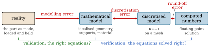
A finite element result differs from what the real part does for three reasons, and Figure 8.20.10 places each between two stages of an analysis. The modelling error is the difference between the real part and the mathematical model we chose for it: the idealised geometry, the supports and loads written as boundary conditions, the material law and the linear assumptions. The discretisation error is the difference between the exact solution of that mathematical model and the solution on the mesh, the error that Mesh convergence watched shrink. The round-off error separates the exact solution of the discretised equations 8.20.1 from the numbers the computer returns, since it calculates with about sixteen significant digits.

The three are rarely of the same size. Round-off is the smallest in a sound model. Solving 8.20.1 loses roughly as many digits as there are in the condition number of \(\bm K\), the ratio of its largest to its smallest eigenvalue. That number grows as the elements shrink and when very stiff and very soft parts are joined in one model, and only an extreme model, a part held so weakly that it is nearly a mechanism or a “rigid” link made a million times stiffer than the material around it, loses the digits we read. The discretisation error is the one we can measure and control, and for the fillet peak of the stepped bar it was about one percent on the mesh with \(h = 0.25~\text{mm}\). The modelling error is usually by far the largest, and no computation on the model reveals it. Suppose the shoulder of the stepped bar is drawn with \(r = 2~\text{mm}\) but machined with a cutter that leaves \(r = 1~\text{mm}\). The converged model of the drawing reports \(K_t\sigma_{\text{nom}}\) with \(K_t = 2.24\), while the part has the factor of 8.19.6 with \(h/r = 5\).

def K_t_step(r):
    """@eq-kt-fit for the stepped flat bar in tension with D = 30 mm and d = 20 mm."""
    q = h_step/r
    return sum((c1 + c2*np.sqrt(q) + c3*q)*(2*h_step/D)**i for i, (c1, c2, c3) in enumerate(c))


ltx(r"K_t(r = 1~\text{mm}) =", K_t_step(1.0), r",\qquad \frac{K_t(1~\text{mm})}{K_t(2~\text{mm})} =",
    K_t_step(1.0)/K_t_step(2.0), precision=3)

The real peak is \(25\) percent higher than the converged model says, an error some twenty times larger than the discretisation error we refined the mesh to remove. A finer mesh reduces only the discretisation error. It solves the same mathematical model more accurately and leaves the gap between the model and the part as it was, so a perfect mesh of a wrong model gives a precise wrong answer. The same holds for a boundary condition. Had we fixed the wide end of the stepped bar, \(u_x = u_y = 0\), instead of letting it slide on the wall, every mesh would have reported singular stresses at the corners of that end, as the fixed bar of Figure 8.20.9 did, and each refinement would have made them larger. The effort of an analysis belongs where the error is: in the idealisation first and in the mesh second.

Verification and validation

The two parts of Figure 8.20.10 are checked in different ways. Verification asks whether we solve the equations right. It compares the computed numbers with the exact solution of the mathematical model, and since that solution is unknown for a real part, it relies on what can be known. Code verification shows that the program reproduces cases with an analytical solution, as our triangles reproduced the chart value \(K_t\) of the filleted shoulder. Solution verification checks the model at hand: a mesh convergence study, equilibrium of the reactions and a hand calculation of the order of magnitude, the checks of the next section. Validation asks whether we solve the right equations. It compares the mathematical model with reality, and that needs a measurement: the force and elongation of the tensile test of Chapter 8.6, the angle of twist measured in the torsion lab, or strain gauges on a prototype. Verification comes first. A disagreement between an unverified model and a test may come from the mesh as much as from the model, so it says nothing about the idealisation. A verified model that agrees with a test has passed for the case tested, and only for that case.

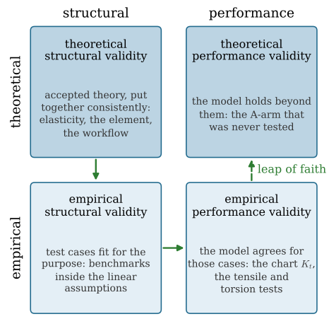
How far a passed test carries over to other cases is the question of the validation square of Pedersen, Emblemsvåg, Bailey, Allen and Mistree [2]. It was proposed for validating design methods and carries over to a finite element model, Figure 8.20.11. It splits validity in two ways. Structural validity concerns whether the method is built correctly and performance validity whether it gives useful results, and each is judged theoretically, in general, and empirically, for chosen example problems. Confidence is built in the order of the arrows. Theoretical structural validity accepts each construct of the method and the consistency of the way they are put together: for us linear elasticity, the element formulation and the workflow of Figure 8.20.1, each inside its stated assumptions. Empirical structural validity accepts that the example problems are fit for the purpose, test cases that resemble the intended use and stay inside the same assumptions, such as the stepped bar for a part with shoulders. Empirical performance validity shows that the model gives the right answer for those examples, against the chart and the lab tests, and that the agreement comes from the model and not from two errors that cancel. Theoretical performance validity, the claim that the model is also right for the A-arm that has never been tested, does not follow from the other three by logic. Pedersen et al. call it a leap of faith, and the other three quadrants are there to make the leap short.

Checking the model

A finite element result is checked before it is believed, and four checks catch most errors.

The first is a hand calculation that gives the order of magnitude, done in minutes with \(F/A\) in a strut, \(My/I\) at the root of an arm, or \(K_t\sigma_{\text{nom}}\) from a chart at a fillet. Where the part is close to the idealisation behind the formula, the model and the formula should agree within tens of percent. A factor of two needs an explanation. A factor of a hundred or a thousand almost never comes from the mechanics. It points to units first, millimetres mixed with metres or newtons with kilonewtons, then to the load, applied a thousand times over or on the wrong face, and then to a boundary condition that holds the part somewhere other than where we think. A model in millimetres with \(E\) entered in pascals is a million times too soft. The stepped bar passed this check against the chart value \(K_t\sigma_{\text{nom}}\) in Mesh convergence.

The second is equilibrium. The reactions at the supports must balance the applied loads, component by component, and every program reports them. A difference means a load lost, a load applied twice, or part of the load going into a support we did not intend. For the stepped bar the wall must take the whole force on the narrow end, \(\sigma_{\text{nom}}\,t\,d/2\) on the half model, and the symmetry line must take no net force.

s = study[2.0][-1]
R_x = s['R'][s['p'] % 2 == 0].sum()                    # the even degrees of freedom are u_x
R_y = s['R'][s['p'] % 2 == 1].sum()
ltx(r"\sum R_x &=", R_x, r"~\text{N}, \qquad -\sigma_{\text{nom}}\,t\,d/2 =", -sigma_nom*t*d/2,
    r"~\text{N}\\ \sum R_y &=", round(R_y, 6) + 0.0, r"~\text{N}", aligned=True, precision=6)

The third is the deformed shape. Plotted with the displacements magnified, it shows at a glance whether the part bends the way we expect, moves where it should be free and stays where it is held. Parts that pass through each other, separate where they are bolted together or stay straight where they should bend reveal a missing connection, a wrong contact or a wrong support. A displacement far larger than a hand estimate suggests a support that is missing or a part that is not connected to the rest.

In an explicit dynamic analysis, of a bumper hitting a wall or a car landing a jump, the energy balance is the check. The total energy, the sum of the kinetic energy, the internal energy stored and dissipated in the material and the smaller contributions of contact and element stabilisation, less the work done by external loads, stays constant through the run. During an impact the kinetic energy turns into internal energy as the structure deforms, and the two curves typically cross while their sum stays flat. A total energy that grows or jumps means energy created by the numerics, often by a contact or by an element distorted beyond what it can represent, and the results after the jump are not to be trusted. The energy absorbed by the stabilisation of reduced-integration elements, the hourglass energy, should remain a small fraction of the internal energy.

These checks are solution verification in the sense of Verification and validation: they show that the equations were solved as intended. Whether the equations describe the real part, with its real supports, loads and material, is validation, and it needs a test, such as a tensile or a torsion test whose measured stiffness the model must reproduce. A hand calculation, a converged mesh and balanced reactions make a test worth running, since they leave the idealisations as the only source of disagreement.

Further reading

Fish and Belytschko give a first course in the method itself, from the rod element to elements in two and three dimensions [3], and Ottosen and Petersson develop it for heat flow and elasticity side by side [4]. Cook, Malkus, Plesha and Witt cover the practice of modelling at greater length, including the choice of elements, error estimates and convergence [5]. Pedersen and co-authors proposed the validation square for design methods, with a discussion of what validating a method can and cannot prove [2]. Williams derived the corner singularities of 8.20.2 for corners of any angle [1]. Björk’s handbook collects the hand formulas that a finite element result should be checked against [6], and Peterson’s charts are the reference for the stress concentration factors a converged model should reproduce [7].