Code
import numpy as np
import sympy as sp
import matplotlib.pyplot as plt
from scipy.optimize import fsolve
from matplotlib.animation import FuncAnimation
from IPython.display import HTML

from mechanicskit import ltx, la, fplot

sp.init_printing()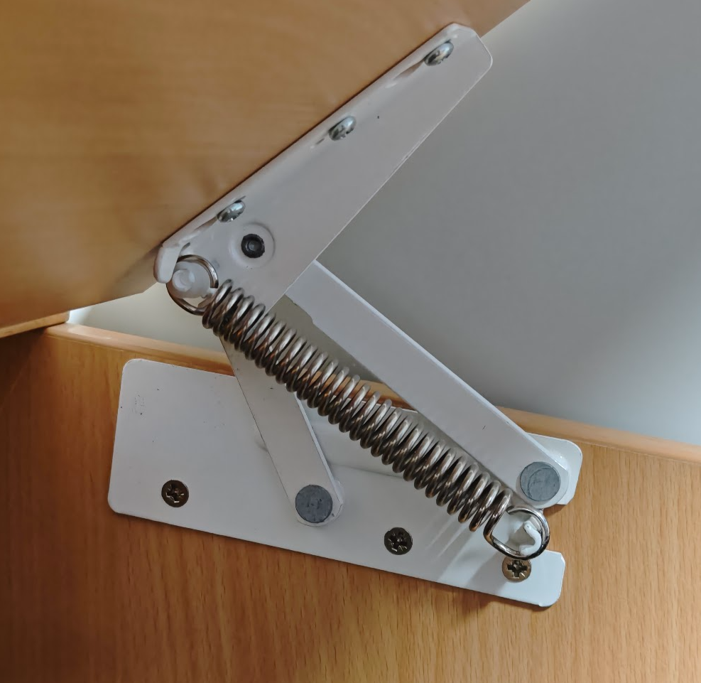
The mechanism in Figure 7.4.1 is the lifting linkage of a paper-bin lid. You can find one on the second floor of JTH; we recommend taking the lid in your hands before reading further. What looks like a simple flap is in fact a four-bar linkage with non-parallel cranks \(OA\) and \(BC\). Because the cranks are unequal in length and tilted with respect to one another, the lid does not rotate about a single fixed axis. It traces a coupler curve instead, a path that lifts the lid up and away from the rim of the bin so the lid never scrapes the opening as it swings. The four-bar layout is what makes that possible.
Your project asks you to redesign this mechanism so the lid closes softly, with no slam at the end of the stroke. To do that you need to know how the lid moves, what its angular velocity and acceleration are at each opening angle, and where the kinetic energy is concentrated as it swings shut. This notebook walks through the model that delivers those quantities. It is the foundation you will build on; the soft-closing logic comes at the end.
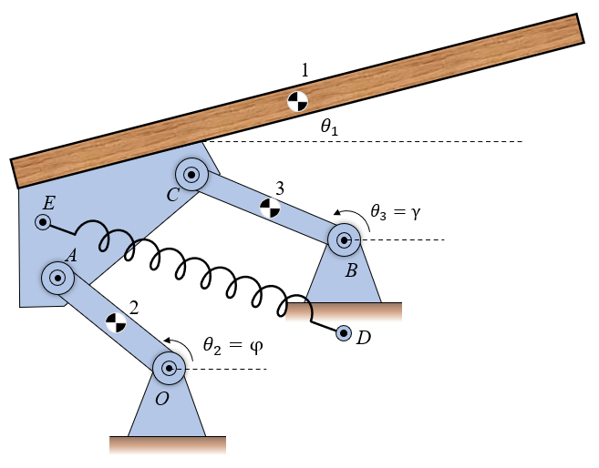
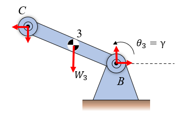
We model the mechanism in 2D as three rigid bodies hinged at four points. The lid is body 1, the coupler of the four-bar. The cranks \(OA\) and \(BC\) (bodies 2 and 3) are the input and output links, both pinned to ground at \(O\) and \(B\). The spring drawn between \(E\) on the lid and the fixed anchor \(D\) stores energy as the lid is opened, but we leave it out of the model in this notebook and add it in your project. Gravity alone drives the motion here.
For any opening angle of the lid we want three quantities: the lid’s angular velocity \(\dot\theta\) and angular acceleration \(\ddot\theta\), the velocity and acceleration of its center of mass \(G_1\), and the time history \(\theta(t)\) when the lid is released from rest and falls under gravity. The lid is taken to be a slender plank of length \(L = 500\) mm. The crank lengths, masses, and pin offsets are read off the actual mechanism, with the understanding that you will refine them in your own design.
import numpy as np
import sympy as sp
import matplotlib.pyplot as plt
from scipy.optimize import fsolve
from matplotlib.animation import FuncAnimation
from IPython.display import HTML
from mechanicskit import ltx, la, fplot
sp.init_printing()The configuration is described by three angles, one per body. The lid’s tilt above horizontal is \(\theta = \theta_1\) (body 1, the coupler); the angle of the crank \(OA\) above horizontal is \(\varphi = \theta_2\) (body 2); the angle of the crank \(BC\) above horizontal is \(\gamma = \theta_3\) (body 3). The mechanism has a single degree of freedom, so \(\varphi\) and \(\gamma\) are determined by \(\theta\) once the geometry is fixed. We set up that closure condition in Section 7.4.3.
The remaining parameters are the crank lengths \(\ell_2 = |OA|\) and \(\ell_3 = |BC|\), the position \(\bm r_{OB}\) of the second ground pivot, the lid length \(L\), and the body-frame offsets that locate the pin \(C\) and the spring anchor \(E\) on the lid.
# Geometry
L      = 0.500          # lid length [m]
l_2    = 0.045          # crank OA length [m]
l_3    = 0.080          # crank BC length [m]
rr_OB  = sp.Matrix([0.060, 0.015, 0])   # fixed-pivot offset O -> B [m]

# Body-frame offsets on the lid, measured from A in the lid's local frame
# (lid lies along its local x-axis when theta = 0)
rr_AC_local = sp.Matrix([0.012, 0.013, 0])     # pin C on lid
rr_AE_local = sp.Matrix([0.004, 0.014, 0])     # spring anchor E on lid
rr_AG1_local = sp.Matrix([L/2,  0.015, 0])     # center of mass G1 (lid midpoint)

# Inertial properties
g    = sp.Rational(981, 100)        # gravity [m/s^2]
m_1  = 0.5                          # lid mass [kg]
m_2  = 0.05                         # crank OA mass [kg]
m_3  = 0.05                         # crank BC mass [kg]
I_1  = m_1 * L**2 / 12              # slender-rod inertia about G1
I_2  = m_2 * l_2**2 / 12
I_3  = m_3 * l_3**2 / 12

ltx(r"L &=", L, r"\\ \ell_2 &=", l_2, r"\\ \ell_3 &=", l_3,
    r"\\ I_1 &=", I_1, r"\;\text{kg}\,\text{m}^2",
    aligned=True)
\[ \begin{aligned}L &=0.50\\ \ell_2 &=0.04\\ \ell_3 &=0.08\\ I_1 &=0.01\;\text{kg}\,\text{m}^2\end{aligned} \]
The closed kinematic chain \(O \to A \to C \to B \to O\) must come back to itself for any valid configuration. Walking from \(O\) via the crank \(OA\) and the lid offset \(AC\) we land at \(C\):
\[ \bm r_{OC}^{(\text{lid path})} = \bm r_{OA}(\varphi) + \bm r_{AC}(\theta). \]
Walking the other way, from \(O\) via the fixed offset \(OB\) and the crank \(BC\), we also land at \(C\):
\[ \bm r_{OC}^{(\text{crank path})} = \bm r_{OB} + \bm r_{BC}(\gamma). \]
Equating the two paths gives the loop equation
\[ \bm r_{OA}(\varphi) + \bm r_{AC}(\theta) - \bm r_{OB} - \bm r_{BC}(\gamma) = \bm 0. \tag{7.4.1}\]
Two scalar equations, three unknowns \((\theta, \varphi, \gamma)\). Picking \(\theta\) as the input collapses 7.4.1 to a \(2\times 2\) nonlinear system in \((\varphi, \gamma)\), which we solve numerically with fsolve. The same construction served the three-bar linkage in the rigid body kinematics chapter; the only difference here is that the coupler \(AC\) has its own angle \(\theta\) rather than being a passive rod.
# Symbolic angles (treated as functions of time so we can differentiate)
t = sp.symbols('t', real=True, positive=True)
theta_f = sp.Function(r'theta')(t)
phi_f   = sp.Function(r'phi')(t)
gamma_f = sp.Function(r'gamma')(t)

# Unit vectors along each link
ee_OA = sp.Matrix([sp.cos(phi_f),   sp.sin(phi_f),   0])  # crank 2
ee_BC = sp.Matrix([sp.cos(gamma_f), sp.sin(gamma_f), 0])  # crank 3

# Position vectors using the angles
rr_OA = l_2 * ee_OA
rr_BC = l_3 * ee_BC

# Lid-frame offsets rotated by theta into the world frame
R_theta = sp.rot_ccw_axis3(theta_f)
rr_AC = R_theta @ rr_AC_local
rr_AE = R_theta @ rr_AE_local
rr_AG1 = R_theta @ rr_AG1_local

# Loop equation (only x and y matter in 2D)
loop = (rr_OA + rr_AC) - (rr_OB + rr_BC)
loop_xy = sp.Matrix([loop[0], loop[1]])
ltx(r"\text{loop equation: } \;", loop_xy, r"= \bm 0")
\[ \text{loop equation: } \;\left[\begin{matrix}- 0.013 \sin{\left(\theta{\left(t \right)} \right)} - 0.08 \cos{\left(\gamma{\left(t \right)} \right)} + 0.045 \cos{\left(\phi{\left(t \right)} \right)} + 0.012 \cos{\left(\theta{\left(t \right)} \right)} - 0.06\\- 0.08 \sin{\left(\gamma{\left(t \right)} \right)} + 0.045 \sin{\left(\phi{\left(t \right)} \right)} + 0.012 \sin{\left(\theta{\left(t \right)} \right)} + 0.013 \cos{\left(\theta{\left(t \right)} \right)} - 0.015\end{matrix}\right]= \bm 0 \]
# Strip the t-dependence so we can lambdify
theta, phi, gamma = sp.symbols('theta phi gamma', real=True)
sub_pos = {theta_f: theta, phi_f: phi, gamma_f: gamma}
loop_xy_alg = loop_xy.subs(sub_pos)

loop_func = sp.lambdify((phi, gamma, theta), loop_xy_alg, 'numpy')

def solve_position(theta_val, guess):
    """Given theta, solve the loop equation for (phi, gamma)."""
    res = fsolve(lambda v: loop_func(v[0], v[1], theta_val).flatten(),
                 guess, full_output=False)
    return res  # [phi, gamma]

# Quick check at theta = 18 deg using a sensible guess
guess0 = np.deg2rad([150.0, 150.0])
phi0, gamma0 = solve_position(np.deg2rad(18.0), guess0)
ltx(r"\varphi|_{\theta=18^\circ} &=", float(np.rad2deg(phi0)), r"^\circ",
    r"\\ \gamma|_{\theta=18^\circ}    &=", float(np.rad2deg(gamma0)), r"^\circ",
    aligned=True, precision=4)
\[ \begin{aligned}\varphi|_{\theta=18^\circ} &=108.6655^\circ\\ \gamma|_{\theta=18^\circ} &=146.8855^\circ\end{aligned} \]
Each pin connecting two bodies is shared by both, so the velocity computed by either body must agree. This is the relative-velocity statement from Section 6.4.3 applied around the same loop we used for position: walking from \(O\) to \(C\) via the lid and via the second crank gives two expressions for \(\bm v_C\), and they must coincide.
For a point on a body rotating about a fixed pivot the velocity is a single cross product. For a point on a body that is itself moving, we add the velocity of a chosen reference point and the relative velocity from that reference. The two paths to \(C\) are
\[ \bm v_C = \underbrace{\bm\omega_{OA}\times\bm r_{OA}}_{\bm v_A} + \underbrace{\bm\omega_{\text{lid}}\times\bm r_{AC}}_{\bm v_{C/A}}, \qquad \bm v_C = \bm 0 + \underbrace{\bm\omega_{BC}\times\bm r_{BC}}_{\bm v_C \text{ (crank 3)}}. \]
With \(\bm\omega_{OA} = \dot\varphi\,\hat{\bm z}\), \(\bm\omega_{\text{lid}} = \dot\theta\,\hat{\bm z}\) and \(\bm\omega_{BC} = \dot\gamma\,\hat{\bm z}\), equating the two paths gives
\[ \dot\varphi\,\hat{\bm z}\times\bm r_{OA} + \dot\theta\,\hat{\bm z}\times\bm r_{AC} - \dot\gamma\,\hat{\bm z}\times\bm r_{BC} = \bm 0. \tag{7.4.2}\]
7.4.2 is linear in the angular rates. Picking \(\dot\theta\) as the input we solve for \(\dot\varphi(\dot\theta, \theta, \varphi, \gamma)\) and \(\dot\gamma(\dot\theta, \theta, \varphi, \gamma)\) symbolically with sp.solve, then lambdify.
# Symbolic angular rates
thetadot, phidot, gammadot = sp.symbols('thetadot phidot gammadot', real=True)
sub_vel = {sp.Derivative(theta_f, t): thetadot,
           sp.Derivative(phi_f,   t): phidot,
           sp.Derivative(gamma_f, t): gammadot}

# Two paths to C
vv_A = sp.Matrix([0, 0, phidot]).cross(rr_OA)
vv_C_via_lid = vv_A + sp.Matrix([0, 0, thetadot]).cross(rr_AC)
vv_C_via_BC  = sp.Matrix([0, 0, gammadot]).cross(rr_BC)

vel_loop = (vv_C_via_lid - vv_C_via_BC).subs(sub_vel).subs(sub_pos)

vel_sol = sp.solve(vel_loop, [phidot, gammadot])
phidot_func   = sp.lambdify((thetadot, theta, phi, gamma), vel_sol[phidot])
gammadot_func = sp.lambdify((thetadot, theta, phi, gamma), vel_sol[gammadot])
ltx(r"\dot\varphi   &=", vel_sol[phidot],
    r"\\ \dot\gamma &=", vel_sol[gammadot], aligned=True)
\[ \begin{aligned}\dot\varphi &=- \dfrac{13.0 \dot{\theta} \sin{\left(\gamma \right)} \sin{\left(\theta \right)}}{- 45.0 \sin{\left(\gamma \right)} \cos{\left(\phi \right)} + 45.0 \sin{\left(\phi \right)} \cos{\left(\gamma \right)}} + \dfrac{12.0 \dot{\theta} \sin{\left(\gamma \right)} \cos{\left(\theta \right)}}{- 45.0 \sin{\left(\gamma \right)} \cos{\left(\phi \right)} + 45.0 \sin{\left(\phi \right)} \cos{\left(\gamma \right)}} - \dfrac{12.0 \dot{\theta} \sin{\left(\theta \right)} \cos{\left(\gamma \right)}}{- 45.0 \sin{\left(\gamma \right)} \cos{\left(\phi \right)} + 45.0 \sin{\left(\phi \right)} \cos{\left(\gamma \right)}} - \dfrac{13.0 \dot{\theta} \cos{\left(\gamma \right)} \cos{\left(\theta \right)}}{- 45.0 \sin{\left(\gamma \right)} \cos{\left(\phi \right)} + 45.0 \sin{\left(\phi \right)} \cos{\left(\gamma \right)}}\\ \dot\gamma &=- \dfrac{13.0 \dot{\theta} \sin{\left(\phi \right)} \sin{\left(\theta \right)}}{- 80.0 \sin{\left(\gamma \right)} \cos{\left(\phi \right)} + 80.0 \sin{\left(\phi \right)} \cos{\left(\gamma \right)}} + \dfrac{12.0 \dot{\theta} \sin{\left(\phi \right)} \cos{\left(\theta \right)}}{- 80.0 \sin{\left(\gamma \right)} \cos{\left(\phi \right)} + 80.0 \sin{\left(\phi \right)} \cos{\left(\gamma \right)}} - \dfrac{12.0 \dot{\theta} \sin{\left(\theta \right)} \cos{\left(\phi \right)}}{- 80.0 \sin{\left(\gamma \right)} \cos{\left(\phi \right)} + 80.0 \sin{\left(\phi \right)} \cos{\left(\gamma \right)}} - \dfrac{13.0 \dot{\theta} \cos{\left(\phi \right)} \cos{\left(\theta \right)}}{- 80.0 \sin{\left(\gamma \right)} \cos{\left(\phi \right)} + 80.0 \sin{\left(\phi \right)} \cos{\left(\gamma \right)}}\end{aligned} \]
A second derivative of the loop equation gives the acceleration relation. The relative-acceleration formula adds a centripetal term to the tangential one,
\[ \bm a_{P/Q} = \bm\alpha\times\bm r_{PQ} + \bm\omega\times(\bm\omega\times\bm r_{PQ}), \]
so the two paths to \(C\) now read
\[ \bm a_C = \bm\alpha_{OA}\times\bm r_{OA} + \bm\omega_{OA}\times(\bm\omega_{OA}\times\bm r_{OA}) + \bm\alpha_{\text{lid}}\times\bm r_{AC} + \bm\omega_{\text{lid}}\times(\bm\omega_{\text{lid}}\times\bm r_{AC}), \]
\[ \bm a_C = \bm\alpha_{BC}\times\bm r_{BC} + \bm\omega_{BC}\times(\bm\omega_{BC}\times\bm r_{BC}). \]
Equating gives a \(2\times 2\) linear system in \(\ddot\varphi\) and \(\ddot\gamma\) once the angles, the angular rates, and \(\ddot\theta\) are known. We solve symbolically once and lambdify, exactly as we did at the velocity stage. Background on the relative-acceleration formula is given in Section 6.4.3.
# Symbolic angular accelerations
thetaddot, phiddot, gammaddot = sp.symbols('thetaddot phiddot gammaddot', real=True)
sub_acc = {sp.Derivative(theta_f, (t, 2)): thetaddot,
           sp.Derivative(phi_f,   (t, 2)): phiddot,
           sp.Derivative(gamma_f, (t, 2)): gammaddot,
           **sub_vel, **sub_pos}

# Helper: rotational acceleration of a body-fixed offset
def aa_rot(omega, alpha, rr):
    wz = sp.Matrix([0, 0, omega])
    az = sp.Matrix([0, 0, alpha])
    return az.cross(rr) + wz.cross(wz.cross(rr))

aa_A = aa_rot(phidot, phiddot, rr_OA)
aa_C_via_lid = aa_A + aa_rot(thetadot, thetaddot, rr_AC)
aa_C_via_BC  = aa_rot(gammadot, gammaddot, rr_BC)

acc_loop = (aa_C_via_lid - aa_C_via_BC).subs(sub_acc)

acc_sol = sp.solve(acc_loop, [phiddot, gammaddot])
phiddot_func   = sp.lambdify((thetaddot, thetadot, theta, phidot, phi, gammadot, gamma),
                             acc_sol[phiddot])
gammaddot_func = sp.lambdify((thetaddot, thetadot, theta, phidot, phi, gammadot, gamma),
acc_sol[gammaddot])We isolate each body and write the planar Newton-Euler equations for it. Pin reactions \(\bm R_O, \bm R_A, \bm R_B, \bm R_C\) appear with opposite signs on the two bodies that share a pin, and gravity acts at each body’s center of mass.
We deliberately leave the spring (and any damper) out of the free body diagrams at this stage. The notebook delivers the kinematic and kinetic skeleton of the mechanism: the angles, velocities, and accelerations as functions of time when only gravity acts. Once that skeleton is verified you plug your own spring and damper in at the relevant pins, which is exactly what your project asks you to do. Including them now would conflate two distinct concerns: getting the mechanism model right, and tuning the closing behaviour.
For each body the translational equation balances forces against the inertial term \(m\,\bm a_{G_i}\), and the rotational equation balances moments about \(G_i\) against \(I_i\,\dot{\bm\omega}_i\). The \(G_i\) accelerations have already been built from the relative-motion machinery above, so plugging them in is mechanical.
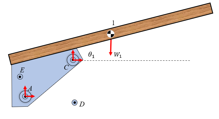
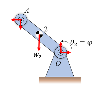
Writing the weight on body \(i\) as \(\bm W_i = -m_i g\,\hat{\bm e}_y\) and taking moments about each body’s center of mass, the Newton-Euler equations for the three bodies read
\[ \begin{aligned} \bm R_A + \bm R_C + \bm W_1 &= m_1\,\bm a_{G_1}, \\ \bm r_{G_1 A}\times\bm R_A + \bm r_{G_1 C}\times\bm R_C &= I_1\,\ddot\theta\,\hat{\bm z}, \end{aligned} \tag{7.4.3}\]
for the lid;
\[ \begin{aligned} \bm R_O - \bm R_A + \bm W_2 &= m_2\,\bm a_{G_2}, \\ \bm r_{G_2 O}\times\bm R_O + \bm r_{G_2 A}\times(-\bm R_A) &= I_2\,\ddot\varphi\,\hat{\bm z}, \end{aligned} \tag{7.4.4}\]
for crank \(OA\); and
\[ \begin{aligned} \bm R_B - \bm R_C + \bm W_3 &= m_3\,\bm a_{G_3}, \\ \bm r_{G_3 B}\times\bm R_B + \bm r_{G_3 C}\times(-\bm R_C) &= I_3\,\ddot\gamma\,\hat{\bm z}, \end{aligned} \tag{7.4.5}\]
for crank \(BC\). The minus signs on \(\bm R_A\) in the crank-\(OA\) equations and on \(\bm R_C\) in the crank-\(BC\) equations are Newton’s third law: the lid pulls back on the crank with the opposite of the force the crank applies to the lid.
# Position vectors of centers of mass
rr_OG2 = (l_2/2) * ee_OA                       # G2 at midpoint of crank OA
rr_OG3 = rr_OB + (l_3/2) * ee_BC               # G3 at midpoint of crank BC
rr_OG1 = rr_OA + rr_AG1                        # G1 on the lid

# Body-relative offsets used in the moment equations
rr_G2O = -(l_2/2) * ee_OA
rr_G2A =  (l_2/2) * ee_OA
rr_G3B = -(l_3/2) * ee_BC
rr_G3C =  (l_3/2) * ee_BC
rr_G1A = -rr_AG1
rr_G1C = rr_AC - rr_AG1

# Time-derivatives of the centers of mass (still as functions of t)
aa_G1 = sp.diff(rr_OG1, t, 2).subs(sub_acc)
aa_G2 = sp.diff(rr_OG2, t, 2).subs(sub_acc)
aa_G3 = sp.diff(rr_OG3, t, 2).subs(sub_acc)

# Strip remaining t-dependence in the offset vectors used below
rr_G2O = rr_G2O.subs(sub_pos); rr_G2A = rr_G2A.subs(sub_pos)
rr_G3B = rr_G3B.subs(sub_pos); rr_G3C = rr_G3C.subs(sub_pos)
rr_G1A = rr_G1A.subs(sub_pos); rr_G1C = rr_G1C.subs(sub_pos)# Pin reactions and weights
R_Ox, R_Oy, R_Ax, R_Ay, R_Bx, R_By, R_Cx, R_Cy = sp.symbols(
'R_Ox R_Oy R_Ax R_Ay R_Bx R_By R_Cx R_Cy', real=True)
RR_O = sp.Matrix([R_Ox, R_Oy, 0])
RR_A = sp.Matrix([R_Ax, R_Ay, 0])
RR_B = sp.Matrix([R_Bx, R_By, 0])
RR_C = sp.Matrix([R_Cx, R_Cy, 0])
WW_1 = sp.Matrix([0, -m_1*g, 0])
WW_2 = sp.Matrix([0, -m_2*g, 0])
WW_3 = sp.Matrix([0, -m_3*g, 0])
# Body 1 (lid): pins A and C act on it; weight at G1
eqF_1 = sp.Eq(RR_A + RR_C + WW_1, m_1 * aa_G1)
eqM_1 = sp.Eq(rr_G1A.cross(RR_A) + rr_G1C.cross(RR_C),
I_1 * sp.Matrix([0, 0, thetaddot]))
# Body 2 (crank OA): pin O and reaction -R_A from the lid; weight at G2
eqF_2 = sp.Eq(RR_O - RR_A + WW_2, m_2 * aa_G2)
eqM_2 = sp.Eq(rr_G2O.cross(RR_O) + rr_G2A.cross(-RR_A),
I_2 * sp.Matrix([0, 0, phiddot]))
# Body 3 (crank BC): pin B and reaction -R_C from the lid; weight at G3
eqF_3 = sp.Eq(RR_B - RR_C + WW_3, m_3 * aa_G3)
eqM_3 = sp.Eq(rr_G3B.cross(RR_B) + rr_G3C.cross(-RR_C),
I_3 * sp.Matrix([0, 0, gammaddot]))Each body contributes one force equation (two scalar components in 2D) and one moment equation (one scalar component in 2D), nine scalar equations across the three bodies in total. The unknowns are the eight pin-reaction components \((R_{Ox}, R_{Oy}, R_{Ax}, R_{Ay}, R_{Bx}, R_{By}, R_{Cx}, R_{Cy})\) and the lid’s angular acceleration \(\ddot\theta\), so the system is square. We hand it to sp.solve and lambdify the resulting expression for \(\ddot\theta\) in terms of the angles, their rates, and the satellite-angle rates \(\dot\varphi, \dot\gamma, \ddot\varphi, \ddot\gamma\), which the velocity and acceleration loops give us in terms of \(\theta, \dot\theta, \ddot\theta\).
equations = [eqF_1, eqM_1, eqF_2, eqM_2, eqF_3, eqM_3]
unknowns  = [R_Ox, R_Oy, R_Ax, R_Ay, R_Bx, R_By, R_Cx, R_Cy, thetaddot]
sol_dyn   = sp.solve(equations, unknowns)

thetaddot_expr = sol_dyn[thetaddot]
thetaddot_func = sp.lambdify(
    (thetadot, theta, phiddot, phidot, phi, gammaddot, gammadot, gamma),
    thetaddot_expr,
)For a given state \((\theta, \dot\theta)\), computing \(\ddot\theta\) takes four steps in order. First we solve the loop equation for \((\varphi, \gamma)\), using the previous step’s solution as initial guess so fsolve lands on the correct branch. With the angles in hand we substitute into the velocity-loop solution to get \((\dot\varphi, \dot\gamma)\), and into the acceleration-loop solution to get \((\ddot\varphi, \ddot\gamma)\), treating \(\ddot\theta\) as the unknown that the kinetics will deliver. Finally we evaluate thetaddot_func to obtain \(\ddot\theta\).
The third step looks circular but is not: the symbolic acceleration loop expresses \(\ddot\varphi, \ddot\gamma\) as linear functions of \(\ddot\theta\), and the kinetics expression \(\ddot\theta = f(\dot\theta, \theta, \dot\varphi, \varphi, \dot\gamma, \gamma, \ddot\varphi, \ddot\gamma)\) closes the loop. Substituting the linear expressions into \(f\) would let us eliminate them up front, but feeding numerical values through one step at a time works equally well.
def dynamics(theta_val, thetadot_val, guess):
    """Return (thetaddot, [phi, gamma]) for the given state."""
    # 1. Position closure
    phi_val, gamma_val = solve_position(theta_val, guess)

    # 2. Velocity closure
    phidot_val   = phidot_func(thetadot_val, theta_val, phi_val, gamma_val)
    gammadot_val = gammadot_func(thetadot_val, theta_val, phi_val, gamma_val)

    # 3. Acceleration closure -- with placeholder thetaddot=0 the loop returns
    #    the part of phiddot/gammaddot that is independent of thetaddot, plus
    #    a coefficient times thetaddot. Since acc_sol is linear in thetaddot,
    #    we evaluate at thetaddot=0 and at thetaddot=1 to get intercept and slope:
    pdd0 = phiddot_func(0.0, thetadot_val, theta_val, phidot_val, phi_val,
                        gammadot_val, gamma_val)
    pdd1 = phiddot_func(1.0, thetadot_val, theta_val, phidot_val, phi_val,
                        gammadot_val, gamma_val)
    gdd0 = gammaddot_func(0.0, thetadot_val, theta_val, phidot_val, phi_val,
                          gammadot_val, gamma_val)
    gdd1 = gammaddot_func(1.0, thetadot_val, theta_val, phidot_val, phi_val,
                          gammadot_val, gamma_val)
    a_p, b_p = pdd1 - pdd0, pdd0   # phiddot   = a_p * thetaddot + b_p
    a_g, b_g = gdd1 - gdd0, gdd0   # gammaddot = a_g * thetaddot + b_g

    # 4. Newton-Euler -- the kinetics expression is also linear in thetaddot
    #    via the inertia of body 1, so we close it the same way. We evaluate
    #    thetaddot_func with both (phiddot, gammaddot) as linear functions of
    #    a candidate thetaddot, and solve the resulting 1D linear equation.
    def f_of_tdd(tdd):
        return thetaddot_func(thetadot_val, theta_val,
                              a_p*tdd + b_p, phidot_val, phi_val,
                              a_g*tdd + b_g, gammadot_val, gamma_val) - tdd
    f0, f1 = f_of_tdd(0.0), f_of_tdd(1.0)
    tdd_sol = -f0 / (f1 - f0)
return tdd_sol, np.array([phi_val, gamma_val])The state is \((\theta, \dot\theta)\). With the dynamics right-hand side in hand we step it forward in time. We use Euler-Cromer (also known as the symplectic or semi-implicit Euler method), which advances the velocity first and then uses the new velocity to advance the position,
\[ \dot\theta_{n+1} = \dot\theta_n + \ddot\theta_n\,\Delta t, \qquad \theta_{n+1} = \theta_n + \dot\theta_{n+1}\,\Delta t. \]
For oscillatory mechanisms Euler-Cromer behaves much better than plain forward Euler: it does not pump energy into the system over long simulations, so a swinging mechanism stays bounded rather than drifting to infinity.
# Initial conditions and time grid
sps   = 1000               # samples per second
t_end = 1.2                # total time [s]
n     = int(t_end * sps)
dt    = 1.0 / sps
time  = np.linspace(0.0, t_end, n)

theta_n     = np.zeros(n)
thetadot_n  = np.zeros(n)
thetaddot_n = np.zeros(n)
phi_n       = np.zeros(n)
gamma_n     = np.zeros(n)

theta_n[0]    = np.deg2rad(18.0)   # release angle
thetadot_n[0] = 0.0                # released from rest
guess         = np.deg2rad([150.0, 150.0])

thetaddot_n[0], guess = dynamics(theta_n[0], thetadot_n[0], guess)
phi_n[0], gamma_n[0]  = guess

# Euler-Cromer loop
for i in range(n - 1):
    tdd, guess = dynamics(theta_n[i], thetadot_n[i], guess)
    thetaddot_n[i+1] = tdd
    thetadot_n[i+1]  = thetadot_n[i] + tdd * dt
    theta_n[i+1]     = theta_n[i]    + thetadot_n[i+1] * dt
phi_n[i+1], gamma_n[i+1] = guessThe three angular quantities tell the story:
fig, axes = plt.subplots(3, 1, figsize=(6, 6), sharex=True)
axes[0].plot(time, np.rad2deg(theta_n), lw=2, color='C0')
axes[0].set_ylabel(r'$\theta$ [deg]'); axes[0].grid(alpha=0.3)
axes[1].plot(time, thetadot_n, lw=2, color='C1')
axes[1].set_ylabel(r'$\dot\theta$ [rad/s]'); axes[1].grid(alpha=0.3)
axes[2].plot(time, thetaddot_n, lw=2, color='C3')
axes[2].set_ylabel(r'$\ddot\theta$ [rad/s$^2$]'); axes[2].set_xlabel(r'$t$ [s]')
axes[2].grid(alpha=0.3)
plt.tight_layout(); plt.show()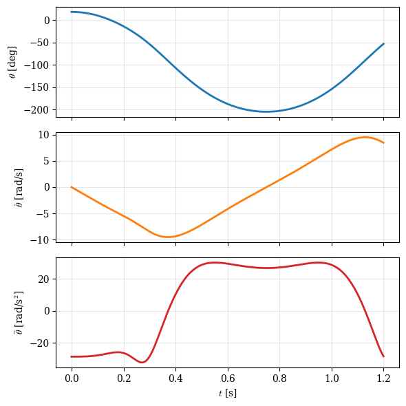
The angles alone are abstract; what the user feels is how fast the tip of the lid is moving when it hits the rim. With a 500 mm lid the tip is at \(\bm r_{A,\text{tip}} = (L, 0)\) in the lid’s body frame. We propagate that point through the simulation and read off the magnitudes of velocity and acceleration. Because the lid translates and rotates together, we use the relative-motion formulas one more time:
\[ \bm v_{\text{tip}} = \bm v_A + \dot\theta\,\hat{\bm z}\times\bm r_{A\text{tip}}, \qquad \bm a_{\text{tip}} = \bm a_A + \ddot\theta\,\hat{\bm z}\times\bm r_{A\text{tip}} + \dot\theta^2(-\bm r_{A\text{tip}}). \]
# Numerical helpers built once
def AB(theta_v, phi_v):
    """Position of A in world frame."""
    return l_2 * np.array([np.cos(phi_v), np.sin(phi_v)])

def vA(thetadot_v, phidot_v, theta_v, phi_v):
    return l_2 * phidot_v * np.array([-np.sin(phi_v), np.cos(phi_v)])

def aA(thetaddot_v, thetadot_v, phiddot_v, phidot_v, theta_v, phi_v):
    tang = l_2 * phiddot_v * np.array([-np.sin(phi_v), np.cos(phi_v)])
    cent = -l_2 * phidot_v**2 * np.array([np.cos(phi_v), np.sin(phi_v)])
    return tang + cent

# Compute phidot, gammadot and phiddot, gammaddot histories
phidot_n   = np.array([phidot_func(thetadot_n[i], theta_n[i], phi_n[i], gamma_n[i])
                        for i in range(n)])
gammadot_n = np.array([gammadot_func(thetadot_n[i], theta_n[i], phi_n[i], gamma_n[i])
                        for i in range(n)])
phiddot_n  = np.array([phiddot_func(thetaddot_n[i], thetadot_n[i], theta_n[i],
                                     phidot_n[i], phi_n[i], gammadot_n[i], gamma_n[i])
                       for i in range(n)])

# Tip speed and acceleration via relative motion
def perp(v):  return np.array([-v[1], v[0]])
tip_local = np.array([L, 0.0])
v_tip = np.zeros(n); a_tip = np.zeros(n)
for i in range(n):
    R = np.array([[np.cos(theta_n[i]), -np.sin(theta_n[i])],
                  [np.sin(theta_n[i]),  np.cos(theta_n[i])]])
    r_AT = R @ tip_local
    vA_i = vA(thetadot_n[i], phidot_n[i], theta_n[i], phi_n[i])
    aA_i = aA(thetaddot_n[i], thetadot_n[i], phiddot_n[i], phidot_n[i], theta_n[i], phi_n[i])
    v_T = vA_i + thetadot_n[i] * perp(r_AT)
    a_T = aA_i + thetaddot_n[i] * perp(r_AT) - thetadot_n[i]**2 * r_AT
    v_tip[i] = np.linalg.norm(v_T)
    a_tip[i] = np.linalg.norm(a_T)

fig, axes = plt.subplots(2, 1, figsize=(6, 4.5), sharex=True)
axes[0].plot(time, v_tip, lw=2, color='C2')
axes[0].set_ylabel(r'$|v_{\mathrm{tip}}|$ [m/s]'); axes[0].grid(alpha=0.3)
axes[1].plot(time, a_tip, lw=2, color='C4')
axes[1].set_ylabel(r'$|a_{\mathrm{tip}}|$ [m/s$^2$]'); axes[1].set_xlabel(r'$t$ [s]')
axes[1].grid(alpha=0.3)
plt.tight_layout(); plt.show()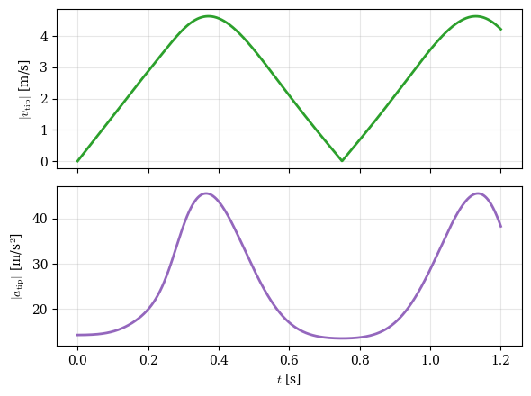
The mechanism is far easier to read as a moving picture than as three plots stacked together. We render the simulation as an embedded HTML5 video. The cranks are line segments; the lid is drawn as a thin rectangle so its rotation is visible.
import matplotlib
matplotlib.rcParams['animation.embed_limit'] = 60

# Downsample to ~25 fps
fps = 25
step = max(1, sps // fps)
idx = np.arange(0, n, step)

# Pre-compute world-frame geometry per frame
OB_xy = np.array([float(rr_OB[0]), float(rr_OB[1])])
A_xy = np.zeros((len(idx), 2))
C_xy = np.zeros((len(idx), 2))
G1_xy = np.zeros((len(idx), 2))
lid_corners = np.zeros((len(idx), 4, 2))   # 4 corners of lid rectangle

# Lid drawn as a thin rectangle of length L, height L_h, anchored near A
L_h = 0.030
local_corners = np.array([[0.0, -L_h/2],
                          [L,   -L_h/2],
                          [L,    L_h/2],
                          [0.0,  L_h/2]])

for k, i in enumerate(idx):
    A_xy[k] = l_2 * np.array([np.cos(phi_n[i]),  np.sin(phi_n[i])])
    C_xy[k] = OB_xy + l_3 * np.array([np.cos(gamma_n[i]), np.sin(gamma_n[i])])
    R = np.array([[np.cos(theta_n[i]), -np.sin(theta_n[i])],
                  [np.sin(theta_n[i]),  np.cos(theta_n[i])]])
    G1_xy[k] = A_xy[k] + R @ np.array([float(rr_AG1_local[0]), float(rr_AG1_local[1])])
    lid_corners[k] = A_xy[k] + (R @ local_corners.T).T

fig, ax = plt.subplots(figsize=(7, 5))
ax.set_aspect('equal')
ax.set_xlim(-0.05, 0.55); ax.set_ylim(-0.05, 0.30)
ax.grid(alpha=0.3); ax.set_xlabel(r'$x$ [m]'); ax.set_ylabel(r'$y$ [m]')

ax.plot(0, 0, 'ks', markersize=10);                 ax.annotate('O', (0, 0),     xytext=(-12, -6), textcoords='offset points')
ax.plot(*OB_xy, 'ks', markersize=10);                ax.annotate('B', OB_xy,      xytext=(8, -6),   textcoords='offset points')

crank_OA, = ax.plot([], [], 'o-', color='C0', lw=3, markersize=6)
crank_BC, = ax.plot([], [], 'o-', color='C3', lw=3, markersize=6)
lid_patch = plt.Polygon(lid_corners[0], closed=True, facecolor='#c8a26a',
                        edgecolor='black', lw=1.2, alpha=0.85)
ax.add_patch(lid_patch)
g1_marker, = ax.plot([], [], 'ko', markersize=5)

def update(k):
    crank_OA.set_data([0, A_xy[k, 0]], [0, A_xy[k, 1]])
    crank_BC.set_data([OB_xy[0], C_xy[k, 0]], [OB_xy[1], C_xy[k, 1]])
    lid_patch.set_xy(lid_corners[k])
    g1_marker.set_data([G1_xy[k, 0]], [G1_xy[k, 1]])
    return crank_OA, crank_BC, lid_patch, g1_marker

anim = FuncAnimation(fig, update, frames=len(idx), interval=1000/fps, blit=False)
plt.close(fig)

video_html = anim.to_html5_video()
video_html = video_html.replace('controls', 'controls autoplay loop muted')
video_html = video_html.replace('<video ', '<video style="width: 100%; height: auto;" ')
HTML(video_html)The simulation above models the lid falling under gravity alone, with no spring force and no damping. The angular velocity at impact is whatever the geometry plus gravity delivers, and it is large. In a real bin you do not want the lid to slam.
A soft closing mechanism shapes the closing stroke so that \(\dot\theta\to 0\) smoothly as \(\theta\to 0\). Two design levers do the work. The first is a spring acting between \(E\) on the lid and \(D\) on the frame: it stores energy as the lid is opened and gives it back during closing, so by choosing its rest length and stiffness you can trade kinetic energy at impact for elastic energy held in the spring. The second is a damper that removes energy from the system, so the lid coasts to a halt rather than bouncing.
Translate “soft closing” into measurable requirements: a maximum impact speed \(|\dot\theta(\theta=0)|\), a maximum tip speed \(|\bm v_{\text{tip}}|\), perhaps a target closing time. Iterate on stiffness and damping until those numbers are met. The kinematic and Newton-Euler skeleton you have here carries both contributions without any restructuring; you only add their forces and moments to body 1 and re-solve.
This is the same spring problem you handled in the Bygeln lab: a linear extension spring between two points, one on the moving body and one on the frame. The same approach applies here, with the only twist being that \(E\) sits in the lid’s body frame and rotates with \(\theta\).
Let \(\bm r_{ED} = \bm r_{OD} - \bm r_{OE}\) be the vector from \(E\) on the lid to the fixed anchor \(D\), \(\ell = \|\bm r_{ED}\|\) the current length, and \(\hat{\bm e}_{ED} = \bm r_{ED}/\ell\) the unit vector along it. A linear extension spring of stiffness \(k\) and rest length \(\ell_0\) pulls the lid toward \(D\) with force
\[ \bm F_s = k(\ell - \ell_0)\,\hat{\bm e}_{ED}. \]
The force enters the Newton-Euler equations of body 1 only. The translational equation in 7.4.3 becomes \(\bm R_A + \bm R_C + \bm W_1 + \bm F_s = m_1\,\bm a_{G_1}\), and the rotational equation picks up the moment \(\bm r_{G_1 E}\times\bm F_s\). The two crank equations are untouched. In code, evaluate \(\bm F_s\) from the current \((\theta, \varphi)\) at each step and add it into eqF_1 and eqM_1 before calling sp.solve.
A damper removes energy in proportion to a velocity. The physically realistic element in this geometry is a linear dashpot between two points, like the spring: a piston-and-cylinder that resists changes in length with a force proportional to its rate of extension. Real soft-close hardware (gas struts, the dampers in cabinet hinges) is built this way. A clean attachment runs from the pin \(C\) on the lid to the fixed pivot \(O\), since \(\bm r_{OC}\) and \(\bm v_C\) both come directly out of the kinematics you already built.
Let \(\ell = \|\bm r_{OC}\|\) be the current length of the dashpot and \(\hat{\bm e}_{OC} = \bm r_{OC}/\ell\) the unit vector along it. The rate of change of length is the projection of \(\bm v_C\) onto \(\hat{\bm e}_{OC}\),
\[ \dot\ell = \hat{\bm e}_{OC}\cdot\bm v_C. \]
A linear dashpot of coefficient \(c_d\) exerts a force on the lid at \(C\) that opposes the relative motion,
\[ \bm F_d = -c_d\,\dot\ell\,\hat{\bm e}_{OC}. \]
The force enters body 1 only. The translational equation in 7.4.3 picks up \(+\bm F_d\) on the left-hand side, and the rotational equation picks up the moment \(\bm r_{G_1 C}\times\bm F_d\). In code, evaluate \(\bm v_C\) from the velocity loop already in place, compute \(\dot\ell\) and \(\bm F_d\), and add to eqF_1 and eqM_1. The coefficient \(c_d\) has units of \(\text{N}\,\text{s}/\text{m}\).
If you want to see the lid decelerate before the dashpot geometry is wired up, the simplest damper to code is a viscous moment on the lid alone, \(\bm M_d = -c\,\dot\theta\,\hat{\bm z}\). It is mathematically clean and unique to a single equation, but it does not correspond to any real machine element at a revolute joint. Use it to confirm the simulator behaves as you expect; switch to the linear dashpot for the report.
The moment enters the rotational equation of body 1 only, \(\bm r_{G_1 A}\times\bm R_A + \bm r_{G_1 C}\times\bm R_C + \bm M_d = I_1\,\ddot\theta\,\hat{\bm z}\). In code, add -c*thetadot to the \(z\) component of eqM_1. The coefficient \(c\) has units of \(\text{N}\,\text{m}\,\text{s}/\text{rad}\).
The mechanism is now yours to redesign. Measure the real bin, refine the masses and inertias, plug in your own spring and damper, and see whether the lid behaves the way you want.