th = np.radians(37.0)                            # any angle
Rc = np.array([[np.cos(th), -np.sin(th)], [np.sin(th), np.cos(th)]])
LTc = np.block([[Rc, np.zeros((2, 2))], [np.zeros((2, 2)), Rc]])   # this is L^T
Kpc = (210e3 * 24 / 500) * np.array([[1, 0, -1, 0], [0, 0, 0, 0],
                                     [-1, 0, 1, 0], [0, 0, 0, 0]])
Kec = LTc @ Kpc @ LTc.T                          # the element seen globally

uc = np.array([0.31, -0.72, 1.14, 0.43])         # any nodal displacements
ur = np.array([2.0, 5.0, 2.0, 5.0])              # a rigid translation
8.13 Systematic truss analysis
“The limitations of the human mind are such that it cannot grasp the behaviour of its complex surroundings and creations in one operation.”
— O. C. Zienkiewicz and R. L. Taylor, The Finite Element Method, 2000
This chapter introduces a systematic approach to analyzing truss structures using the direct stiffness method, see e.g., [1], [2], and [3]. The objective is to express equilibrium and compatibility in linear algebra form (\(\mathbf{K u = f}\)), assemble element contributions into a global system, and implement the entire pipeline in python code.
This skill is foundational for upcoming courses where we implement our own Finite Element Methods and is essential for understanding the numerics behind the FEA software we use. The emphasis is on numerical formulation rather than structural analysis by hand, using clear data structures, robust assembly, reproducible solvers, and automated post-processing.
Introduction to truss analysis
A truss is a structural assembly composed of slender members connected at joints, where each member is assumed to carry only axial forces (tension or compression). The approach we develop here is known as the direct stiffness method [2,3], which forms the basis of modern matrix structural analysis.
The essence of our approach lies in recognizing that any truss element, regardless of its orientation in space, behaves locally as a simple one-dimensional rod. By establishing a transformation between local element coordinates and global structural coordinates, we can systematically assemble the global stiffness matrix and solve for nodal displacements. From these displacements, we recover member forces, stresses, and strains: the quantities that mechanical engineers need for design and analysis.
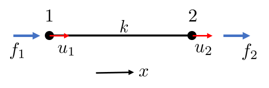
Figure 8.13.1 is the element everything else is built from.
The one-dimensional rod element
We begin with the simplest structural element: a one-dimensional rod of length \(L\), cross-sectional area \(A\), and Young’s modulus \(E\). When the rod is aligned with its axis (the local \(x'\)-direction), the relationship between the axial force \(N\) and the displacement difference between its two ends follows directly from Hooke’s law:
\[ N=k \underbrace{\left(u_2-u_1\right)}_\delta \]
here, we recognize the difference in displacement at the deformation of the rod, i.e., \[ \delta = u_2 - u_1 \]
furthermore, the element stiffness is given by \(k=\frac{EA}{L}\).
With \(N=f_2\) and \(f_1=-N\), we can write
\[ \left\{\begin{array}{l} f_2=k\left(u_2-u_1\right) \\ f_1=k\left(u_1-u_2\right) \end{array}\right. \]
or on matrix form
\[ k\left[\begin{array}{cc} 1 & -1 \\ -1 & 1 \end{array}\right]\left[\begin{array}{l} u_1 \\ u_2 \end{array}\right]=\left[\begin{array}{l} f_1 \\ f_2 \end{array}\right] \]
or
\[ \mathbf{K}_e \mathbf{u}=\mathbf{f} \]
Element stiffness matrix in local coordinates
Now, consider some arbitrary rod in a two dimensional setting, as in Figure 8.13.2.
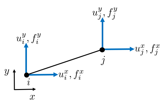
Each node can be translated in the x- and y-direction and each node can carry loads in x- and y-directions.
To formulate the element equations systematically, we introduce the concept of the element stiffness matrix. In local coordinates, each element has four degrees of freedom: two displacement components at each end node. However, for a rod that carries only axial loads, the transverse components (perpendicular to the rod axis) do not participate in the force-displacement relationship.
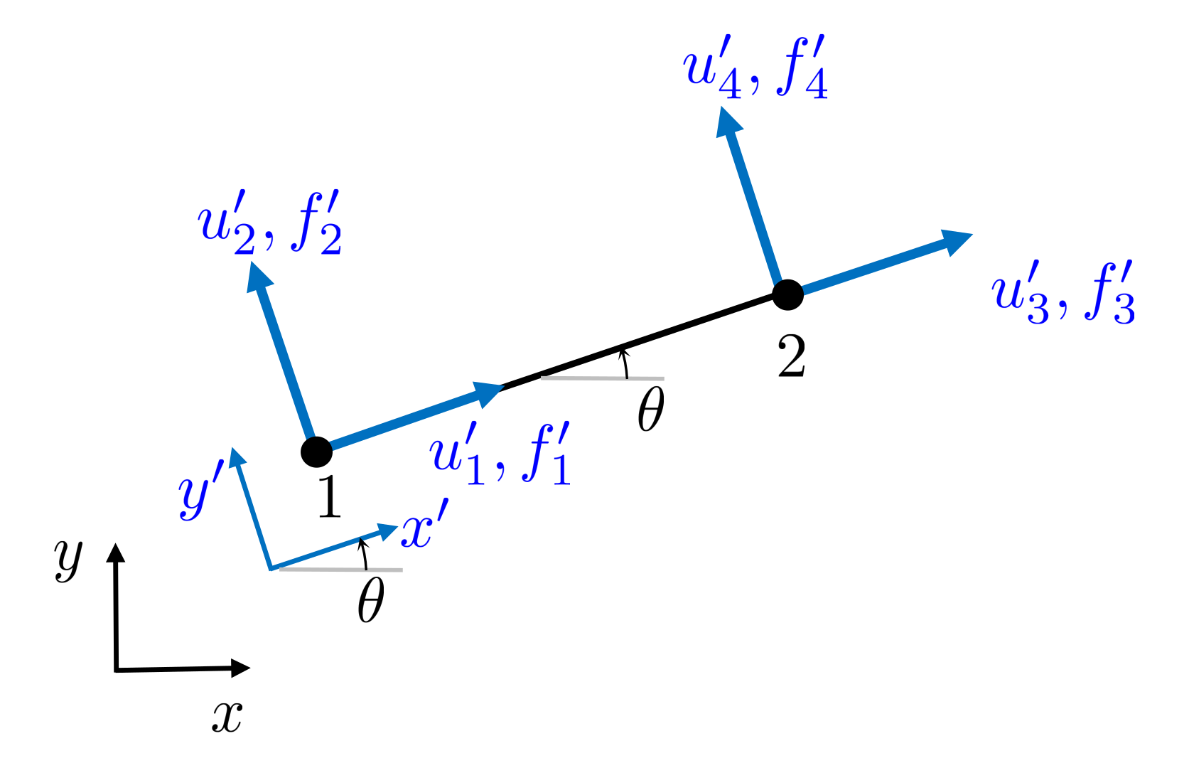
As Figure 8.13.3 shows, each rod has a local coordinate system \(x'\) and \(y'\) and local node numbers 1 and 2. The local coordinate system is rotated compared to the global coordinate system, and the angle is denoted by \(\theta\). In the local coordinates we have
\[ \begin{cases}k\left(u_1'-u_3'\right) & =f_1' \\ 0 & =f_2^{\prime} \\ k\left(u_3^{\prime}-u_1^{\prime}\right) & =f_3^{\prime} \\ 0 & =f_4^{\prime}\end{cases} \]
where indices 1 and 2 refer to the first node (axial and transverse directions), and indices 3 and 4 refer to the second node. The above relation can be written on matrix form:
\[ k\left[\begin{array}{cccc} 1 & 0 & -1 & 0 \\ 0 & 0 & 0 & 0 \\ -1 & 0 & 1 & 0 \\ 0 & 0 & 0 & 0 \end{array}\right]\left[\begin{array}{c} u_1^{\prime} \\ u_2^{\prime} \\ u_3^{\prime} \\ u_4^{\prime} \end{array}\right]=\left[\begin{array}{c} f_1^{\prime} \\ f_2^{\prime} \\ f_3^{\prime} \\ f_4^{\prime} \end{array}\right] \]
or
\[ \boxed{\mathbf{K}'_e \mathbf{u}'_e = \mathbf{f}'_e} \tag{8.13.1}\]
where the local element stiffness matrix is:
\[ \mathbf{K}'_e = k \begin{bmatrix} 1 & 0 & -1 & 0 \\ 0 & 0 & 0 & 0 \\ -1 & 0 & 1 & 0 \\ 0 & 0 & 0 & 0 \end{bmatrix} \]
Note that this matrix is singular (has zero determinant) because two degrees of freedom are unconstrained. This is expected for a rod element that has no stiffness in the transverse direction.
Coordinate Transformation
In a 2D truss, individual rod elements can be oriented at any angle, meaning their natural axial direction will likely not align with the global X and Y axes used for the overall structure. This misalignment requires us to express the stiffness of each element in the global frame before they can be combined into a global stiffness. We achieve this by applying a coordinate transformation to each element’s local stiffness matrix. By rotating the local stiffness properties into the global system, we can systematically assemble the contributions from all elements to form the stiffness matrix for the entire truss.
Figure 8.13.4 shows the two frames and the angle between them.
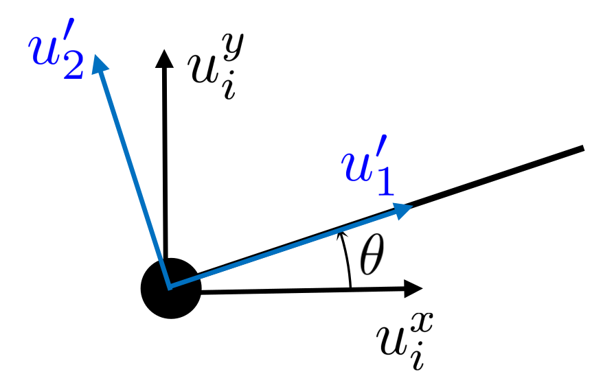
Consider a truss element oriented at an arbitrary angle \(\theta\) with respect to the global \(x\)-axis. The local coordinate system \((x', y')\) is aligned with the rod axis, while the global system \((x, y)\) is fixed in space. We need a relation between \(\mathbf{u}_e^{\prime}\) and \(u_i\) and \(u_j\). The local entities of each rod need to be expressed in terms of global coordinates for unification, i.e., such that we can combine them into a structure. Let’s express the local displacements in terms of global displacements using the angle \(\theta\):
\[ \left\{\begin{array}{l} u_i^x=u_1^{\prime} \cos \theta-u_2^{\prime} \sin \theta \\ u_i^y=u_1^{\prime} \sin \theta+u_2^{\prime} \cos \theta \\ u_j^x=u_3^{\prime} \cos \theta-u_4^{\prime} \sin \theta \\ u_j^y=u_3^{\prime} \sin \theta+u_4^{\prime} \cos \theta \end{array}\right. \]
writing things in matrix form allows us to uncover matrices with interesting properties, we rewrite the equations above on matrix form:
\[ \left[\begin{array}{c} u_i^x \\ u_i^y \\ u_j^x \\ u_j^y \end{array}\right]=\left[\begin{array}{cccc} \cos \theta & -\sin \theta & 0 & 0 \\ \sin \theta & \cos \theta & 0 & 0 \\ 0 & 0 & \cos \theta & -\sin \theta \\ 0 & 0 & \sin \theta & \cos \theta \end{array}\right]\left[\begin{array}{c} u_1^{\prime} \\ u_2^{\prime} \\ u_3^{\prime} \\ u_4^{\prime} \end{array}\right] \]
here that matrix is known as the transformation matrix \(\mathbf L^\mathsf T\), we can write the expression more compactly as
\[ \mathbf{u}_e=\mathbf{L}^T \mathbf{u}_e^{\prime} \]
The transformation matrix
The displacement components in global coordinates \((u, v)\) relate to local coordinates \((u', v')\) through the rotation transformation:
\[ \begin{bmatrix} u' \\ v' \end{bmatrix} = \begin{bmatrix} \cos\theta & \sin\theta \\ -\sin\theta & \cos\theta \end{bmatrix} \begin{bmatrix} u \\ v \end{bmatrix} \]
This rotation matrix transforms displacement vectors from global to local coordinates. For the complete element with two nodes (four degrees of freedom), we construct the transformation matrix \(\mathbf{L}\) by applying the rotation to each node:
\[ \boxed{\mathbf{L} = \begin{bmatrix} \cos\theta & \sin\theta & 0 & 0 \\ -\sin\theta & \cos\theta & 0 & 0 \\ 0 & 0 & \cos\theta & \sin\theta \\ 0 & 0 & -\sin\theta & \cos\theta \end{bmatrix}} \]
An important property of this matrix is that it is orthogonal, meaning:
\[ \mathbf{L}^\mathsf{T} \mathbf{L} = \mathbf{L} \mathbf{L}^\mathsf{T} = \mathbf{I} \quad \text{and} \quad \mathbf{L}^{-1} = \mathbf{L}^\mathsf{T} \]
This orthogonality has profound physical significance. The strain energy stored in a deformed element is given by \(U = \frac{1}{2}\mathbf{u}^\mathsf{T}\mathbf{K}\mathbf{u}\). Since a rotation is merely a change in perspective (how we describe the same physical configuration), the energy must remain unchanged regardless of which coordinate system we use. Mathematically, the orthogonality of \(\mathbf{L}\) ensures that the quadratic form \(\mathbf{u}^\mathsf{T}\mathbf{K}\mathbf{u}\) is preserved under the transformation, meaning the calculated strain energy is identical whether computed in local or global coordinates. This consistency is essential: if the energy changed with coordinate system choice, our analysis would yield different results depending on an arbitrary modeling decision rather than the underlying physics.
It is worth working out the energy on an example. With \(\mathbf u' = \mathbf L\mathbf u\) and \(\mathbf K_e = \mathbf L^\mathsf{T}\mathbf K'_e\mathbf L\),
\[ U = \tfrac{1}{2}\mathbf u^\mathsf{T}\mathbf K_e\mathbf u = \tfrac{1}{2}\mathbf u^\mathsf{T}\mathbf L^\mathsf{T}\mathbf K'_e\mathbf L\mathbf u = \tfrac{1}{2}(\mathbf L\mathbf u)^\mathsf{T}\mathbf K'_e(\mathbf L\mathbf u) = \tfrac{1}{2}\mathbf u'^\mathsf{T}\mathbf K'_e\mathbf u' = U' \]
The two frames therefore agree for every \(\mathbf u\), not only for well chosen ones. The check below takes an element at an arbitrary angle with an arbitrary set of nodal displacements, and adds a rigid translation, which moves both nodes alike and so must store nothing at all.
\[ U = 9252.947967,\quad U' = 9252.947967,\quad U_{\mathrm{rigid}} = 0.000000 \]
Using the transformation matrix we can transform local quantities to global
\[ \mathbf{u}_e=\mathbf{L}^\mathsf{T} \mathbf{u}_e^{\prime} \Leftrightarrow \mathbf{u}_e^{\prime}=\mathbf{L} \mathbf{u}_e \tag{8.13.2}\]
and
\[ \mathbf{f}_e=\mathbf{L}^\mathsf{T} \mathbf{f}_e^{\prime} \Leftrightarrow \mathbf{f}_e^{\prime}=\mathbf{L} \mathbf{f}_e \tag{8.13.3}\]
Inserting (8.13.2) and (8.13.3) into the global equilibrium equation (8.13.1) gives
\[ \mathbf{L}^\mathsf{T} \mathbf{K}_e^{\prime} \mathbf{L} \mathbf{u}_e=\mathbf{f}_e \]
or
\[ \mathbf{K}_e \mathbf{u}_e=\mathbf{f}_e \]
where \(\mathbf{K}_e\) is known as the element stiffness matrix in global coordinates.
\[ \boxed{\mathbf{K}_e = \mathbf{L}^\mathsf{T} \mathbf{K}'_e \mathbf{L}} \]
How to compute the transformation matrix \(\mathbf L^\mathsf T\)
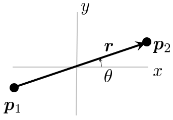
A clever computational trick avoids the need to explicitly compute angles. Given the coordinates of the two nodes defining an element, as in Figure 8.13.5, we can compute the rod vector \(\mathbf{r} = \mathbf{p}_2 - \mathbf{p}_1\) and normalize it:
\[ \hat{\mathbf{r}}=\frac{\mathbf{r}}{|\mathbf{r}|}=\left[\begin{array}{c} \cos \theta \\ \sin \theta \end{array}\right]=:\left[\begin{array}{c} c \\ s \end{array}\right] \]
such that we get
\[ \mathbf{L}^T=\left[\begin{array}{cccc} c & -s & 0 & 0 \\ s & c & 0 & 0 \\ 0 & 0 & c & -s \\ 0 & 0 & s & c \end{array}\right] \]
Carrying out this matrix multiplication with \(c = \cos\theta\) and \(s = \sin\theta\), we obtain the explicit form of the global element stiffness matrix:
\[ \mathbf{K}_e = k \begin{bmatrix} c^2 & cs & -c^2 & -cs \\ cs & s^2 & -cs & -s^2 \\ -c^2 & -cs & c^2 & cs \\ -cs & -s^2 & cs & s^2 \end{bmatrix} \]
This matrix is symmetric, as required for a conservative mechanical system. It also has a beautiful structure: the diagonal \(2 \times 2\) blocks are identical, and the off-diagonal blocks are their negatives, reflecting the action-reaction principle.
Post-processing: member quantities
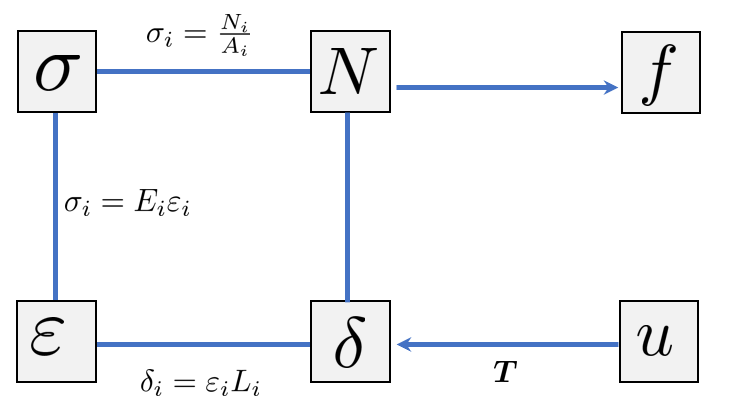
After solving for nodal displacements, we need to recover the member forces and stresses. These quantities are essential for structural design. The key insight is that the member deformation (elongation) can be extracted directly from the global displacement vector. Figure 8.13.6 is the road we travel to get there.
Element deformation
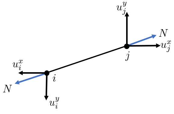
The deformation of an element is the change in its length, which corresponds to the relative displacement of its end nodes in the axial direction. From Figure 8.13.7 we can see that the deformation of the rod is
\[ \delta=\Delta u=\left(u_j^x \cos \theta+u_j^y \sin \theta\right)-\left(u_i^x \cos \theta+u_i^y \sin \theta\right) \]
This can be written om matrix form as
\[ \delta=\underbrace{\left[\begin{array}{llll} -c & -s & c & s \end{array}\right]}_{\mathbf{T}}\left[\begin{array}{c} u_i^x \\ u_i^y \\ u_j^x \\ u_j^y \end{array}\right]=\mathbf{T} \cdot \mathbf{u}_e \]
where \(\mathbf T\) is known as the transformation vector that projects the nodal displacements onto the rod axis direction. We thus have
\[ \boxed{\delta = \mathbf{T} \cdot \mathbf{u}_e} \]
Member force
The axial force in the member follows directly from the deformation:
\[ \boxed{N = k \delta = \frac{EA}{L} \mathbf{T} \cdot \mathbf{u}_e} \]
A positive value indicates tension, while a negative value indicates compression.
Strain and stress
The engineering strain is the deformation divided by the original length:
\[ \boxed{\varepsilon = \frac{\delta}{L}} \]
Note that the length of the element \(L\) can be computed from the nodal coordinates as
\[ L = |\mathbf r| = | \mathbf p_j - \mathbf p_i | \]
The axial stress follows from Hooke’s law or directly from the force:
\[ \boxed{\sigma = \frac{N}{A} = E\varepsilon} \]
These relationships allow us to assess whether the structure remains within acceptable stress limits and to understand the load paths through the truss.
Element load vector (or reaction force vector)
\[ \mathbf{f}^e=\mathbf{T}^T N=k \mathbf{T}_{4 \times 1}^T \mathbf{T}_{1 \times 4} \mathbf{u}_{4 \times 1}^e=k\left[\begin{array}{c} -c \\ -s \\ c \\ s \end{array}\right]\left[\begin{array}{llll} -c & -s & c & s \end{array}\right]\left[\begin{array}{c} u_i^x \\ u_i^y \\ u_j^x \\ u_j^y \end{array}\right] \]
or
\[ \left[\begin{array}{l} f_i^x \\ f_i^y \\ f_j^x \\ f_j^y \end{array}\right]=\underbrace{\frac{E A}{L}\left[\begin{array}{cccc} c^2 & c s & -c^2 & -c s \\ c s & s^2 & -c s & -s^2 \\ -c^2 & -c s & c^2 & c s \\ c s & -s^2 & c s & s^2 \end{array}\right]}_{\mathbf{K}_e}\left[\begin{array}{c} u_i^x \\ u_i^y \\ u_j^x \\ u_j^y \end{array}\right] \]
Implementation in Python
Now we translate this theoretical framework into a computational workflow. The implementation follows the conceptualize-formulate-compute-analyze pattern that characterizes modern computational mechanics. We shall use SymPy for symbolic manipulation and NumPy for numerical computation, allowing us to see both the mathematical structure and the numerical results.
Symbolic derivation of element stiffness
Let us first verify the element stiffness matrix transformation symbolically. This provides confidence in our implementation and reveals the mathematical structure.
import sympy as sp

# Define symbolic variables
theta, k = sp.symbols("theta k", real=True, positive=True)
c, s = sp.cos(theta), sp.sin(theta)

# Local element stiffness matrix (template)
K_prime = k * sp.Matrix([[1, 0, -1, 0],
                         [0, 0, 0, 0],
                         [-1, 0, 1, 0],
                         [0, 0, 0, 0]])
\[ \mathbf{k} = \left[\begin{matrix}k & 0 & - k & 0\\0 & 0 & 0 & 0\\- k & 0 & k & 0\\0 & 0 & 0 & 0\end{matrix}\right] \]
# Transformation matrix (L^T maps global to local)
L_T = sp.Matrix([[c, -s, 0, 0],
                 [s, c, 0, 0],
                 [0, 0, c, -s],
                 [0, 0, s, c]])
\[ \mathbf{L}^\mathsf{T} = \left[\begin{matrix}\cos{\left(\theta \right)} & - \sin{\left(\theta \right)} & 0 & 0\\\sin{\left(\theta \right)} & \cos{\left(\theta \right)} & 0 & 0\\0 & 0 & \cos{\left(\theta \right)} & - \sin{\left(\theta \right)}\\0 & 0 & \sin{\left(\theta \right)} & \cos{\left(\theta \right)}\end{matrix}\right] \]
Let’s verify the orthogonality property of the transformation matrix:
# Verify L^T * L = I
identity_check = sp.trigsimp(L_T * L_T.T)
identity_check
\(\displaystyle \left[\begin{matrix}1 & 0 & 0 & 0\\0 & 1 & 0 & 0\\0 & 0 & 1 & 0\\0 & 0 & 0 & 1\end{matrix}\right]\)
As expected, we obtain the identity matrix, confirming orthogonality. Now we compute the global element stiffness:
# Global element stiffness: K_e = L^T * K'_e * L
K_e = sp.trigsimp(L_T.T * K_prime * L_T)
\[ \mathbf{K}_e = \left[\begin{matrix}k \cos^{2}{\left(\theta \right)} & - \dfrac{k \sin{\left(2 \theta \right)}}{2} & - k \cos^{2}{\left(\theta \right)} & \dfrac{k \sin{\left(2 \theta \right)}}{2}\\- \dfrac{k \sin{\left(2 \theta \right)}}{2} & k \sin^{2}{\left(\theta \right)} & \dfrac{k \sin{\left(2 \theta \right)}}{2} & - k \sin^{2}{\left(\theta \right)}\\- k \cos^{2}{\left(\theta \right)} & \dfrac{k \sin{\left(2 \theta \right)}}{2} & k \cos^{2}{\left(\theta \right)} & - \dfrac{k \sin{\left(2 \theta \right)}}{2}\\\dfrac{k \sin{\left(2 \theta \right)}}{2} & - k \sin^{2}{\left(\theta \right)} & - \dfrac{k \sin{\left(2 \theta \right)}}{2} & k \sin^{2}{\left(\theta \right)}\end{matrix}\right] \]
Verification at special angles
To build confidence in our derivation, let’s evaluate the global stiffness matrix at specific angles where we can verify the result by inspection.
# At theta = 0 (horizontal rod)
K_e_0 = K_e.subs(theta, 0)
K_e_0
\(\displaystyle \left[\begin{matrix}k & 0 & - k & 0\\0 & 0 & 0 & 0\\- k & 0 & k & 0\\0 & 0 & 0 & 0\end{matrix}\right]\)
For \(\theta = 0\), the rod is horizontal, so the axial direction aligns with the global \(x\)-axis. The stiffness matrix shows coupling only in the \(x\)-direction (local degrees of freedom 1 and 3), which is exactly what we expect.
# At theta = 90 degrees (vertical rod)
K_e_90 = K_e.subs(theta, sp.pi / 2)
K_e_90
\(\displaystyle \left[\begin{matrix}0 & 0 & 0 & 0\\0 & k & 0 & - k\\0 & 0 & 0 & 0\\0 & - k & 0 & k\end{matrix}\right]\)
For \(\theta = 90°\), the rod is vertical, and the stiffness couples only the \(y\)-direction displacements (local degrees of freedom 2 and 4). This confirms our transformation is working correctly.
Example 1: Complete truss solver in 2D, Python implementation
We implement the complete truss analysis following a systematic workflow: define geometry, assemble global stiffness, apply boundary conditions, solve for displacements, and compute member quantities.
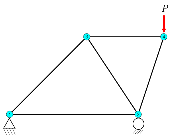
Let us analyze the structure of Figure 8.13.8 as an example and look at the implementation details in python.
import numpy as np
import matplotlib.pyplot as plt
from mechanicskit import OneArray, draw_truss, ltx

# Node coordinates [x, y] in mm. Row i is node i.
nodes = OneArray(np.array([
    [0, 0],      # Node 1
    [500, 0],    # Node 2
    [300, 300],  # Node 3
    [600, 300],  # Node 4
], dtype=float))

# Element connectivity, by node number. Row e is element e.
elements = OneArray(np.array([
    [1, 2],  # Element 1: node 1 to node 2
    [1, 3],  # Element 2
    [2, 3],  # Element 3
    [2, 4],  # Element 4
    [3, 4],  # Element 5
]))
Problem statement:
Given the structure above, determine all displacements, member forces, deformations, strains and stresses as well as reaction forces in the supports.
Solution
The coordinates are given by the variable nodes and elements defines the node connectivity. The order of the columns in elements is not important.
Both are OneArray, so they are numbered the way the figure is numbered: nodes[3] is the third node and elements[5] is the fifth element. There is no row that has to be counted from zero, and no -1 anywhere in what follows.
Using the topological data from above, we can draw the truss ourselves. Figure 8.13.9 is made from the two tables and nothing else, so it is worth comparing against Figure 8.13.8 before going any further: if a support or an arrow is in the wrong place, the tables are wrong.
fig, ax = plt.subplots(figsize=(7, 4))
draw_truss(nodes, elements, presc=[1, 2, 4], loads=[[4, 0, -10e3]], ax=ax)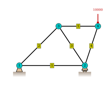
The total number of degrees of freedom (or equations), \(n_{\text {dof }}\) is given by
\[ n_{\mathrm{dof}}=n_{\mathrm{nod}} \cdot n_{\mathrm{loc}}=4 \cdot 2=8 \]
where \(n_{\text {nod }}\) is the number of nodes and \(n_{\text {loc }}\) is the number of local degrees of freedom per node.
The global displacement field and load field are given by
\[ \mathbf{u}=\left[\begin{array}{c} u_1^x=0 \\ u_1^y=0 \\ u_2^x \\ u_2^y=0 \\ u_3^x \\ u_3^y \\ u_4^x \\ u_4^y \end{array}\right], \mathbf{f}=\left[\begin{array}{c} f_1^x=0 \\ f_1^y=0 \\ f_2^x=0 \\ f_2^y=0 \\ f_3^x=0 \\ f_3^y=0 \\ f_4^x=0 \\ f_4^y=-P \end{array}\right] \]
With the resulting linear system taking the form of
\[ \mathbf{K}_{8 \times 8} \mathbf{u}_{8 \times 1}=\mathbf{f}_{8 \times 1} \tag{8.13.4}\]
The unknown displacements are computed by establishing the global stiffness matrix (system matrix) \(\mathbf K\). Creating the linear system (8.13.4), applying boundary conditions, and solving for \(\mathbf u\). This is done by the following steps:
- Initialize the global stiffness matrix \(\mathbf{K}\) as an \(n_{\text {dof }} \times n_{\text {dof }}\) zero matrix.
- Loop over each element to compute its contribution to the global stiffness matrix:
- Extract the node indices and coordinates for the current element.
- Compute the length and orientation of the element.
- Construct the transformation matrix \(\mathbf{L}\).
- Compute the local stiffness matrix \(\mathbf{K}'_e\).
- Transform to global coordinates to obtain \(\mathbf{K}_e\).
- Assemble \(\mathbf{K}_e\) into the global stiffness matrix \(\mathbf{K}\) at the appropriate indices.
- Add the element load vector to the global load vector.
- Apply boundary conditions by modifying \(\mathbf{K}\) and \(\mathbf{f}\) to account for fixed supports.
- Solve the modified linear system for the unknown displacements \(\mathbf{u}\).
Step by step implementation
We begin with some preliminaries and initialize the global system matrix and vectors using the number of degrees of freedom.
nele = len(elements)  # number of elements
nnod = len(nodes)     # number of nodes
ndofs = nnod * 2      # 2 DOF per node (u_x, u_y)

K = OneArray(np.zeros((ndofs, ndofs)))  # Global stiffness matrix
f = OneArray(np.zeros(ndofs))           # Global force vector
u = OneArray(np.zeros(ndofs))           # Global displacement vector
Kprime = np.array([[1, 0, -1, 0], [0, 0, 0, 0], [-1, 0, 1, 0], [0, 0, 0, 0]])
Ltot = 0                                # Total length of truss
E = OneArray(210000 * np.ones(nele))    # Young's modulus in MPa
A = OneArray(4 * 6 * np.ones(nele))     # Cross-sectional area in mm^2
Element 1
We begin by computing which global degrees of freedom correspond to our first element.
iel = 1               # Element number
n1, n2 = elements[iel]  # Nodes for this element
Node numbers for element 1 are: n1=1 and n2=2.
Node \(i\) owns two degrees of freedom, one per direction: \(2i-1\) is its \(x\) and \(2i\) is its \(y\). The data structure of dofs is the same as for the displacements and loads above.
# DOF numbers for the first element
dofs = [2 * n1 - 1, 2 * n1, 2 * n2 - 1, 2 * n2]
Degree of freedom numbers for element 1 are: [np.int64(1), np.int64(2), np.int64(3), np.int64(4)].
Computing the element stiffness matrix
p1 = nodes[n1]  # node coordinates
p2 = nodes[n2]  # node coordinates
Coordinates of the nodes of element 1 are: p1=[0. 0.] and p2=[500. 0.].
r = p2 - p1 # element vector
Element vector for element 1 is: r=[500. 0.].
L = np.linalg.norm(r) # element length
The length of element 1 is: L=500.0.
er = r / L # unit vector along element
The unit vector along element 1 is: er=[1. 0.].
c, s = er[0], er[1] # direction cosines
The cosine and sine of element 1 are: c=1.0, s=0.0.
R = np.array([[c, -s], [s, c]])
The rotation matrix for element 1 is:
\[ \mathbf R = \begin{bmatrix}1.0000 & -0.0000 \\ 0.0000 & 1.0000\end{bmatrix} \]
LT = np.block([[R, np.zeros((2, 2))], [np.zeros((2, 2)), R]])\[ \mathbf L^\mathsf{T} = \begin{bmatrix}1.0000 & -0.0000 & 0.0000 & 0.0000 \\ 0.0000 & 1.0000 & 0.0000 & 0.0000 \\ 0.0000 & 0.0000 & 1.0000 & -0.0000 \\ 0.0000 & 0.0000 & 0.0000 & 1.0000\end{bmatrix} \]
Ai = A[iel]
Ei = E[iel]
ki = Ei * Ai / L
Ke = ki * LT @ Kprime @ LT.T\[ \mathbf K_e = \begin{bmatrix}10080 & 0 & -10080 & 0 \\ 0 & 0 & 0 & 0 \\ -10080 & 0 & 10080 & 0 \\ 0 & 0 & 0 & 0\end{bmatrix} \]
Assembly process
The element stiffness matrix \(\mathbf K_e\) needs to be added to the global stiffness matrix \(\mathbf K\) at the correct locations corresponding to the global degrees of freedom of the element. This process is known as assembly. We append (add) the stiffness contributions using the following code:
K[dofs, dofs] += Ke takes the rows and columns of the global stiffness matrix K that belong to the degrees of freedom of this element, and adds the element matrix into that submatrix. A OneArray reads a pair of index lists the way the mathematics does, as the submatrix on those rows and columns, so the line is the same as
\[ \mathbf K([\,\text{dofs}\,],[\,\text{dofs}\,]) \mathrel{{+}{=}} \mathbf K_e \]
The += is what makes this assembly rather than assignment: a degree of freedom shared by several elements is written to more than once, and every visit adds to what is already there.
K[dofs, dofs] += Ke\[ \mathbf K = \begin{bmatrix}10080 & 0 & -10080 & 0 & 0 & 0 & 0 & 0 \\ 0 & 0 & 0 & 0 & 0 & 0 & 0 & 0 \\ -10080 & 0 & 10080 & 0 & 0 & 0 & 0 & 0 \\ 0 & 0 & 0 & 0 & 0 & 0 & 0 & 0 \\ 0 & 0 & 0 & 0 & 0 & 0 & 0 & 0 \\ 0 & 0 & 0 & 0 & 0 & 0 & 0 & 0 \\ 0 & 0 & 0 & 0 & 0 & 0 & 0 & 0 \\ 0 & 0 & 0 & 0 & 0 & 0 & 0 & 0\end{bmatrix} \]
This is the simplest form of assembly in code. It is easy to read and understand. It is however not very efficient for very large problems with hundreds of thousands of elements. So there exists other methods of dealing with this. But that is a topic for a course in high performance computing.
The rest of the elements are dealt with in an automated manner by executing the above lines of code for each element number, iel. This is done using the for loop:
nele = len(elements)  # number of elements
nnod = len(nodes)     # number of nodes
ndofs = nnod * 2      # 2 DOF per node (u_x, u_y)

K = OneArray(np.zeros((ndofs, ndofs)))  # Global stiffness matrix
f = OneArray(np.zeros(ndofs))           # Global force vector
u = OneArray(np.zeros(ndofs))           # Global displacement vector
Kprime = np.array([[1, 0, -1, 0], [0, 0, 0, 0], [-1, 0, 1, 0], [0, 0, 0, 0]])
Ltot = 0                                # Total length of truss
E = OneArray(210000 * np.ones(nele))    # Young's modulus in MPa
A = OneArray(4 * 6 * np.ones(nele))     # Cross-sectional area in mm^2

for iel, (n1, n2) in enumerate(elements, start=1):
    r = nodes[n2] - nodes[n1]
    L = np.linalg.norm(r)
    Ltot += L
    c, s = r / L
    R = np.array([[c, -s], [s, c]])
    LT = np.block([[R, np.zeros((2, 2))], [np.zeros((2, 2)), R]])
    Ai = A[iel]
    Ei = E[iel]
    ki = Ei * Ai / L
    Ke = ki * LT @ Kprime @ LT.T
    dofs = [2 * n1 - 1, 2 * n1, 2 * n2 - 1, 2 * n2]
    K[dofs, dofs] += Ke
\[ \mathbf K = \begin{bmatrix}16020 & 5940 & -10080 & 0 & -5940 & -5940 & 0 & 0 \\ 5940 & 5940 & 0 & 0 & -5940 & -5940 & 0 & 0 \\ -10080 & 0 & 15975 & -1670 & -4301 & 6452 & -1594 & -4781 \\ 0 & 0 & -1670 & 24021 & 6452 & -9677 & -4781 & -14344 \\ -5940 & -5940 & -4301 & 6452 & 27041 & -512 & -16800 & 0 \\ -5940 & -5940 & 6452 & -9677 & -512 & 15617 & 0 & 0 \\ 0 & 0 & -1594 & -4781 & -16800 & 0 & 18394 & 4781 \\ 0 & 0 & -4781 & -14344 & 0 & 0 & 4781 & 14344\end{bmatrix} \]
This code block is the cornerstone of the systematic truss analysis. It automates the assembly of the global stiffness matrix by iterating over each element, computing its local stiffness matrix, transforming it to global coordinates, and adding it to the appropriate locations in the global matrix. This loop encapsulates the essence of the direct stiffness method, allowing us to handle complex truss structures with ease.
Applying boundary conditions and solving the system
The resulting system \(\mathbf {K u = f}\), however, is singular, meaning it cannot be solved directly. In mechanical terms, the structure contains rigid body rotations or translations that are not constrained by supports. To resolve this, we apply boundary conditions by modifying the global stiffness matrix and load vector to account for fixed supports. This typically involves removing rows and columns corresponding to constrained degrees of freedom.
The reduction above is written for supports that hold a degree of freedom at zero. A prescribed displacement that is non-zero needs one extra term, because the column of \(\mathbf K\) belonging to that degree of freedom no longer multiplies a zero. Splitting the system into free and prescribed degrees of freedom,
\[ \begin{bmatrix} \mathbf K_{ff} & \mathbf K_{fp} \\ \mathbf K_{pf} & \mathbf K_{pp} \end{bmatrix} \begin{bmatrix} \mathbf u_f \\ \mathbf u_p \end{bmatrix} = \begin{bmatrix} \mathbf f_f \\ \mathbf f_p \end{bmatrix} \]
the first row gives the reduced system that we actually solve,
\[ \boxed{\mathbf K_{ff}\, \mathbf u_f = \mathbf f_f - \mathbf K_{fp}\, \mathbf u_p} \]
so the known displacements move to the right-hand side as an equivalent load. They act exactly like a reaction force: imposing a displacement on a spring is the same as applying whatever force produces it. Setting \(\mathbf u_p = \mathbf 0\) makes the extra term vanish and recovers the simple reduction used above, which is why zero supports can be handled by deleting rows and columns and nothing else.
Figure 8.13.10 animates the two steps on a six degree of freedom truss in which \(u_2^y\) is prescribed. The column \([K_{12}, \ldots, K_{62}]^\mathsf{T}\) is multiplied by the known \(u_2^y\) and carried across to the right-hand side, and only then are the row and column belonging to that degree of freedom struck out.
The order matters. Deleting the row and column first would silently discard the load that the prescribed displacement imposes on the rest of the structure, and the remaining displacements would come out as though the support had not moved at all. We apply the full treatment in Section 8.13.8 at the end of this chapter.
We assign the known boundary conditions and loads, reading them off Figure 8.13.8.
# Node 1 is pinned, so both of its degrees of freedom are held.
# Node 2 sits on a roller, so only its y is held and DOF 3 stays free.
presc = [1, 2, 4]      # Prescribed DOF numbers
u[presc] = 0.0         # Prescribed displacements in mm

# Loads: node 4 is pulled down, which is its y degree of freedom, number 8
f[2 * 4] = -10000.0    # Load in N at node 4 in the negative y-direction

free = [k for k in range(1, ndofs + 1) if k not in presc]

u[free] = np.linalg.solve(K[free, free], f[free])
\[ \mathbf u = \begin{bmatrix}0.0000 \\ 0.0000 \\ -0.1984 \\ 0.0000 \\ 0.2467 \\ 0.0901 \\ 0.4451 \\ -0.9116\end{bmatrix} \]
We can separate the x- and y-components of the displacements into a two column matrix for easier handling in the visualization step below.
U = OneArray(u.data.reshape((nnod, 2)))\[ \mathbf U = \begin{bmatrix}0.0000 & 0.0000 \\ -0.1984 & 0.0000 \\ 0.2467 & 0.0901 \\ 0.4451 & -0.9116\end{bmatrix} \]
Visualization of results
Visualization is essential for understanding structural behavior. We plot the deformed shape (with amplification for visibility) and color-code the members according to their stress levels.
UR = OneArray(np.hypot(U.data[:, 0], U.data[:, 1]))\[ \mathbf{UR} = \begin{bmatrix}0.0000 \\ 0.1984 \\ 0.2626 \\ 1.0145\end{bmatrix} \]
Figure 8.13.11 shows the result, drawn far larger than it really is so that the shape can be seen at all.
Code
fig, ax = plt.subplots(figsize=(7, 4.5))
draw_truss(nodes, elements, presc=presc, loads=f, displacements=U, scale=80, ax=ax)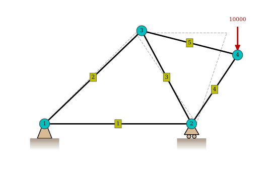
A single picture at one scale factor hides how much of the shape is the scale factor and how much is the truss. Figure 8.13.12 grows the scale from nothing instead. Growing the scale from nothing settles that: every joint moves along a straight line from where it started, and the ones that are held do not move at all.
Code
from mechanicskit import animate_truss, to_responsive_html

anim = animate_truss(nodes, elements, U, presc=presc, loads=f,
                     scale_max=80, frames=20, figsize=(6.4, 3.6))
to_responsive_html(anim, container_id="truss-deformation", autoplay=False)Computing member quantities
Once the displacements have been computed we can compute the normal forces, resultant forces, deformations, strains and stresses.
React = OneArray(np.zeros(ndofs))  # Reaction forces, two DOF per node
delta = OneArray(np.zeros(nele))   # Element deformations
N = OneArray(np.zeros(nele))       # Normal forces in the elements
epsilon = OneArray(np.zeros(nele)) # Strains in the elements
sigma = OneArray(np.zeros(nele))   # Stresses in the elements

for iel, (n1, n2) in enumerate(elements, start=1):
    r = nodes[n2] - nodes[n1]
    L = np.linalg.norm(r)
    c, s = r / L
    T = np.array([-c, -s, c, s])

    Ai = A[iel]
    Ei = E[iel]
    ki = Ei * Ai / L

    dofs = [2 * n1 - 1, 2 * n1, 2 * n2 - 1, 2 * n2]

    ue = u[dofs]
    delta[iel] = T @ ue
    N[iel] = ki * delta[iel]
    epsilon[iel] = delta[iel] / L
    sigma[iel] = N[iel] / Ai

    React[dofs] += N[iel] * T

# One row per node, its x and y reaction side by side
R = OneArray(React.data.reshape((nnod, 2)))
\[ \mathbf{R} = \begin{bmatrix}0 & -2000 \\ -0 & 12000 \\ -0 & -0 \\ 0 & -10000\end{bmatrix} \]
Visualize element results on deformed shape
The same deformed shape carries four different stories depending on what we colour it by: stress in Figure 8.13.13, normal force in Figure 8.13.14, elongation in Figure 8.13.15 and strain in Figure 8.13.16. The member numbers are left off so that the values can be read instead.
Code
fig, ax = plt.subplots(figsize=(7.5, 4.5))
draw_truss(nodes, elements, presc=presc, displacements=U, scale=80,
           values=sigma.data, value_label="Stress [MPa]", cmap="jet",
           element_numbers=False, ax=ax)
moved = nodes.data + 80 * U.data
for iel, (n1, n2) in enumerate(elements, start=1):
    mid = (moved[n1 - 1] + moved[n2 - 1]) / 2
    v = sigma[iel]
    ax.text(*mid, f"$\\sigma={v:.2f}$ MPa", ha="center", va="center", fontsize=8,
            bbox=dict(boxstyle="square,pad=0.2", facecolor="w", edgecolor="none"))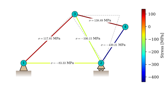
Code
fig, ax = plt.subplots(figsize=(7.5, 4.5))
draw_truss(nodes, elements, presc=presc, displacements=U, scale=80,
           values=N.data, value_label="Element force [N]", cmap="jet",
           element_numbers=False, ax=ax)
moved = nodes.data + 80 * U.data
for iel, (n1, n2) in enumerate(elements, start=1):
    mid = (moved[n1 - 1] + moved[n2 - 1]) / 2
    v = N[iel]
    ax.text(*mid, f"$N={v:.0f}$ N", ha="center", va="center", fontsize=8,
            bbox=dict(boxstyle="square,pad=0.2", facecolor="w", edgecolor="none"))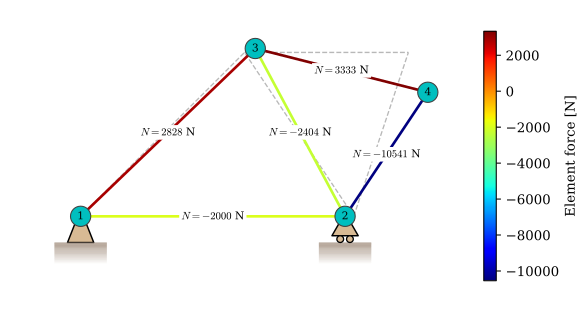
Code
fig, ax = plt.subplots(figsize=(7.5, 4.5))
draw_truss(nodes, elements, presc=presc, displacements=U, scale=80,
           values=delta.data, value_label="Element deformation [mm]", cmap="jet",
           element_numbers=False, ax=ax)
moved = nodes.data + 80 * U.data
for iel, (n1, n2) in enumerate(elements, start=1):
    mid = (moved[n1 - 1] + moved[n2 - 1]) / 2
    v = delta[iel]
    ax.text(*mid, f"$\\delta={v:.3f}$ mm", ha="center", va="center", fontsize=8,
            bbox=dict(boxstyle="square,pad=0.2", facecolor="w", edgecolor="none"))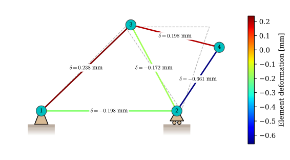
Code
fig, ax = plt.subplots(figsize=(7.5, 4.5))
draw_truss(nodes, elements, presc=presc, displacements=U, scale=80,
           values=epsilon.data, value_label="Element strain [%]", cmap="jet",
           element_numbers=False, ax=ax)
moved = nodes.data + 80 * U.data
for iel, (n1, n2) in enumerate(elements, start=1):
    mid = (moved[n1 - 1] + moved[n2 - 1]) / 2
    v = epsilon[iel]
    ax.text(*mid, f"$\\varepsilon={v*100:.3f}$ %", ha="center", va="center", fontsize=8,
            bbox=dict(boxstyle="square,pad=0.2", facecolor="w", edgecolor="none"))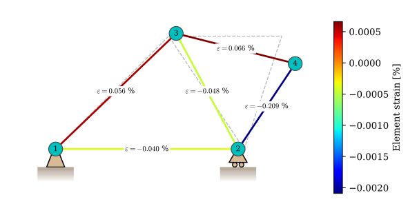
Example 2: prescribed displacements
Here, in addition for nodal forces, we also have nodes with prescribed displacements which are non-zero. This is the same as deforming a spring to a certain length, it will correspond to a force, but we control the displacement instead. Figure 8.13.17 is the structure we solve.
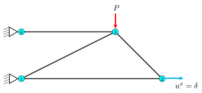
Given: \(\delta=1\) mm. \(P=10\) kN.
Find the deformed shape, member forces and reaction force in node 2.
# Node coordinates [x, y] in mm. Row i is node i.
nodes = OneArray(np.array([
    [0, 0],      # Node 1
    [600, 0],    # Node 2
    [400, 200],  # Node 3
    [0, 200],    # Node 4
], dtype=float))

# Element connectivity, by node number. Row e is element e.
elements = OneArray(np.array([
    [1, 2],  # Element 1
    [3, 4],  # Element 2
    [1, 3],  # Element 3
    [3, 2],  # Element 4
]))
Initiate variables
nele = len(elements)  # number of elements
nnod = len(nodes)     # number of nodes
ndofs = nnod * 2      # 2 DOF per node (u_x, u_y)

K = OneArray(np.zeros((ndofs, ndofs)))  # Global stiffness matrix
f = OneArray(np.zeros(ndofs))           # Global force vector
u = OneArray(np.zeros(ndofs))           # Global displacement vector
Kprime = np.array([[1, 0, -1, 0], [0, 0, 0, 0], [-1, 0, 1, 0], [0, 0, 0, 0]])
Ltot = 0                                # Total length of truss
E = OneArray(210000 * np.ones(nele))    # Young's modulus in MPa
A = OneArray(4 * 6 * np.ones(nele))     # Cross-sectional area in mm^2
Drawing it from the tables again, Figure 8.13.18 shows node 2 held in \(x\) only, so it is free to slide vertically while we push it sideways.
Code
fig, ax = plt.subplots(figsize=(7, 3.6))
draw_truss(nodes, elements, presc=[1, 2, 3, 7, 8], loads=[[3, 0, -10e3]], ax=ax)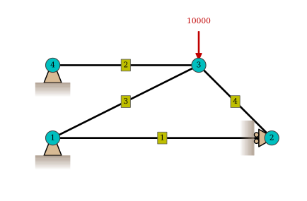
for iel, (n1, n2) in enumerate(elements, start=1):
    r = nodes[n2] - nodes[n1]
    L = np.linalg.norm(r)
    Ltot += L
    c, s = r / L
    R = np.array([[c, -s], [s, c]])
    LT = np.block([[R, np.zeros((2, 2))], [np.zeros((2, 2)), R]])
    Ai = A[iel]
    Ei = E[iel]
    ki = Ei * Ai / L
    Ke = ki * LT @ Kprime @ LT.T
    dofs = [2 * n1 - 1, 2 * n1, 2 * n2 - 1, 2 * n2]
    K[dofs, dofs] += Ke
delta = 1.0 # the prescribed displacement, in mm
# Node 1 is pinned (DOF 1 and 2). Node 2 is on a roller and pushed sideways,
# so its x, DOF 3, is prescribed to delta. Node 4 is pinned (DOF 7 and 8).
presc = [1, 2, 3, 7, 8]
u[presc] = [0.0, 0.0, delta, 0.0, 0.0]
# Loads: node 3 is pulled down, which is its y degree of freedom, number 6
f[2 * 3] = -10000.0
free = [k for k in range(1, ndofs + 1) if k not in presc]
# The prescribed column no longer multiplies a zero, so it moves to the right
fr = K[free, presc] @ u[presc]
u[free] = np.linalg.solve(K[free, free], f[free] - fr)U = OneArray(u.data.reshape((nnod, 2)))\[ \mathbf U = \begin{bmatrix}0.0000 & 0.0000 \\ 1.0000 & -8.1985 \\ 1.5873 & -7.6112 \\ 0.0000 & 0.0000\end{bmatrix} \]
UR = OneArray(np.hypot(U.data[:, 0], U.data[:, 1]))\[ \mathbf{UR} = \begin{bmatrix}0.0000 \\ 8.2593 \\ 7.7750 \\ 0.0000\end{bmatrix} \]
React = OneArray(np.zeros(ndofs))  # Reaction forces, two DOF per node
delta_e = OneArray(np.zeros(nele)) # Element deformations
N = OneArray(np.zeros(nele))       # Normal forces in the elements
epsilon = OneArray(np.zeros(nele)) # Strains in the elements
sigma = OneArray(np.zeros(nele))   # Stresses in the elements

for iel, (n1, n2) in enumerate(elements, start=1):
    r = nodes[n2] - nodes[n1]
    L = np.linalg.norm(r)
    c, s = r / L
    T = np.array([-c, -s, c, s])

    ki = E[iel] * A[iel] / L
    dofs = [2 * n1 - 1, 2 * n1, 2 * n2 - 1, 2 * n2]

    delta_e[iel] = T @ u[dofs]
    N[iel] = ki * delta_e[iel]
    epsilon[iel] = delta_e[iel] / L
    sigma[iel] = N[iel] / A[iel]

    React[dofs] += N[iel] * T

R = OneArray(React.data.reshape((nnod, 2)))
\[ \mathbf{R} = \begin{bmatrix}11600 & 10000 \\ 8400 & 0 \\ 0 & -10000 \\ -20000 & 0\end{bmatrix} \]
Figure 8.13.19 shows what the pushed truss settles into. Node 2 has moved the millimetre we asked of it and has dropped as well, since nothing holds it vertically, while nodes 1 and 4 have not moved at all.
Code
fig, ax = plt.subplots(figsize=(7.5, 4))
draw_truss(nodes, elements, presc=presc, displacements=U, scale=5,
           values=N.data, value_label="Normal force [N]", cmap="jet", ax=ax)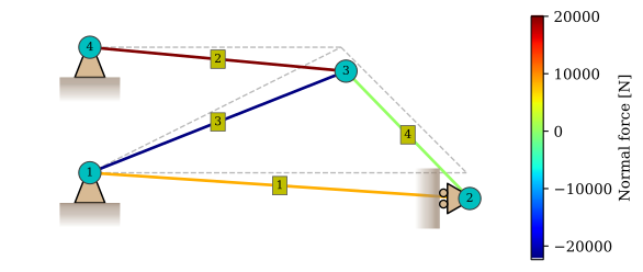
Further reading
The direct stiffness method for truss structures follows standard treatments in structural mechanics textbooks. For further reading on matrix methods in structural analysis, see [3], [4], [5], and [2]. A comprehensive treatment of the finite element method, which builds upon these matrix methods, can be found in [6], [1], and [7].
References
[1]
Ottosen NS, Petersson H. Introduction to the finite element method. New York etc.: Prentice Hall; 1992.
[2]
Przemieniecki JS. Theory of matrix structural analysis. 1st ed. McGraw-Hill; 1968.
[3]
McGuire W, Gallagher RH, Ziemian RD. Matrix structural analysis. 2nd ed. John Wiley & Sons; 2000.
[4]
Kassimali A. Matrix analysis of structures. 2nd ed. Cengage Learning; 2012.
[5]
Hibbeler RC. Structural analysis. 8th ed. Prentice Hall; 2012.
[6]
Felippa CA. Introduction to finite element methods. University of Colorado at Boulder; 2004.
[7]
Cook RD, Malkus DS, Plesha ME, Witt RJ. Concepts and applications of finite element analysis, 4th edition. 4th ed. Wiley; 2001.