“Equal weights at equal distances are in equilibrium, and equal weights at unequal distances are not in equilibrium but incline towards the weight which is at the greater distance.”
— Archimedes, On the Equilibrium of Planes, Book I, Postulate 1, translated by T. L. Heath, 1897
Center of mass – Analytical
The weights \(\bm W_i = -W_i\bm e_z\) are parallel, so their total moment equals that of the total weight \(W = \sum W_i\) acting at \(\bar{\bm r}\),
here \(V\) denotes volume but can also be area or line length.
For general bodies we need to add up all small weight, masses, or spatial elements, forming an integral
\[
\bar{\boldsymbol r} = \frac{\int \boldsymbol r \, dV}{\int dV} = \frac{\int \boldsymbol r \, dV}{V}
\]
Center of mass – Composite areas
Most cross sections we meet in machine elements are built from rectangles, triangles and circular parts whose areas and centroids are known. The sums above then apply directly, with the volumes \(V_i\) replaced by the areas \(A_i\) of the parts,
\[
\bar x = \frac{\sum A_i x_i}{\sum A_i}, \quad \bar y = \frac{\sum A_i y_i}{\sum A_i},
\]
where \((x_i, y_i)\) is the centroid of part \(i\). A hole enters as a part with negative area, so a plate with a bore is the full plate minus a circle. The bookkeeping is a table with one row per part and the columns \(A_i\), \(x_i\), \(y_i\), \(A_i x_i\) and \(A_i y_i\), and the column sums give the centroid.
The sketcher below builds that table from a drawing. Shapes snap to each other’s corners, edges and centres, every dimension can be clicked and given a new value, and the centroid \(C\) follows as we edit. It opens with a T-section of a \(120 \cdot 20\) mm flange on a \(20 \cdot 80\) mm web with a \(\varnothing 12\) mm bore at mid-height of the web, whose centroid lies on the line of symmetry at \(\bar y = 70.87\) mm. Ticking second moments adds the parallel-axis table that we need later for beams, and Copy as Python gives the same table in SymPy with exact values.
In practice, we use a CAD system to compute the center of mass, since the analytical approach is tedious even for slightly complex object and practically impossible for anything moderately complex.
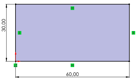
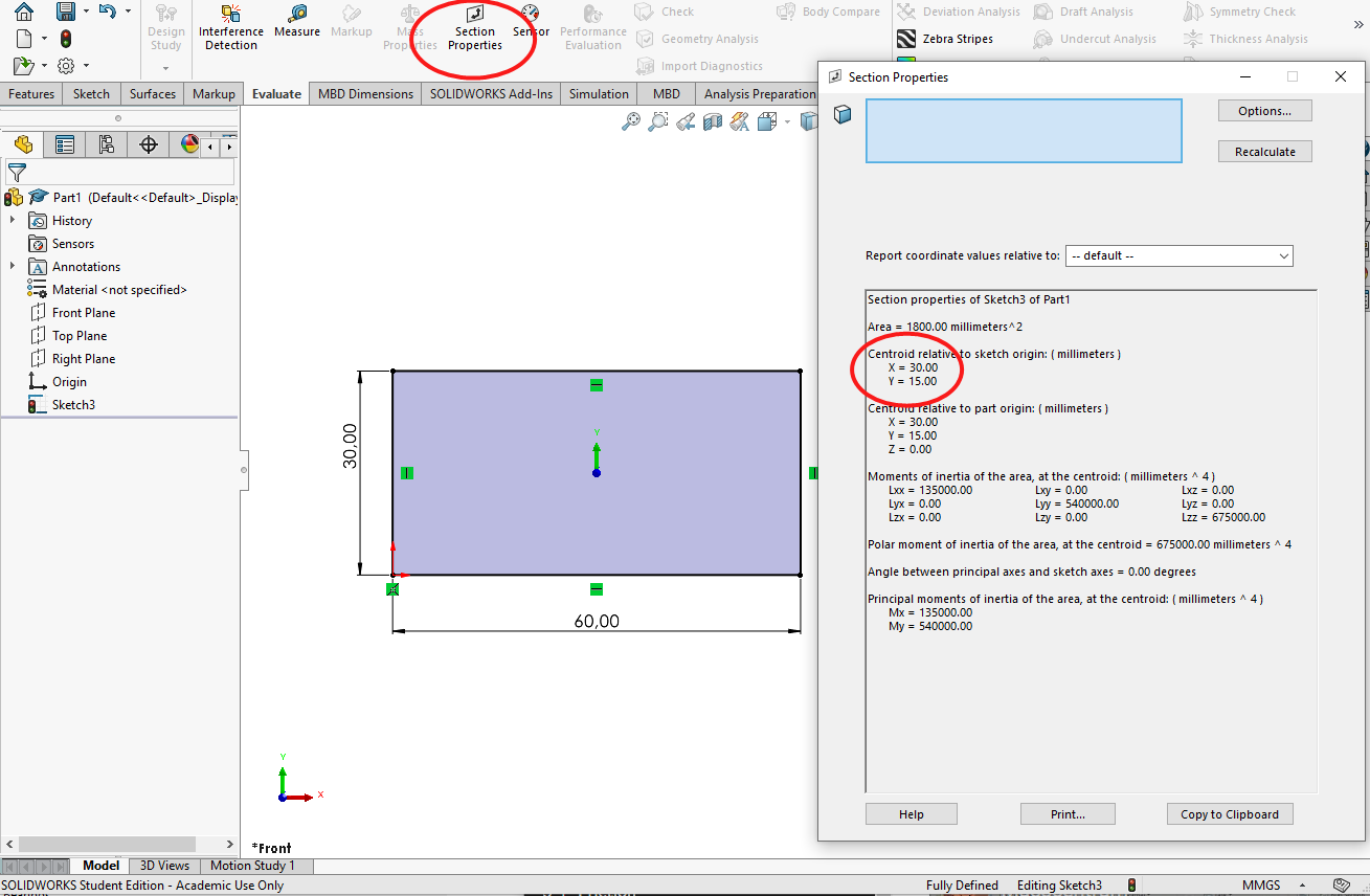
For this simple 2D shape the origin is in the lower left corner and thus the center of mass is at \(x=30\)mm and \(y=15\)mm. We can determine this using SolidWorks, by creating the sketch as a closed shape and going to Evaluate and Section Properties.
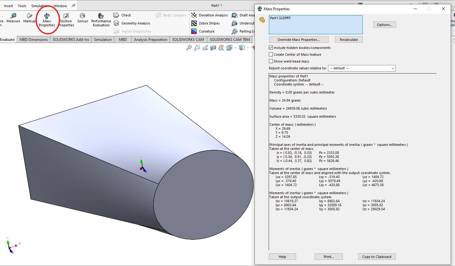
For three dimensional objects such as this below
we go to Evaluate and Mass Properties where we get all geometrical properties, we shall return to this tool in later chapters.
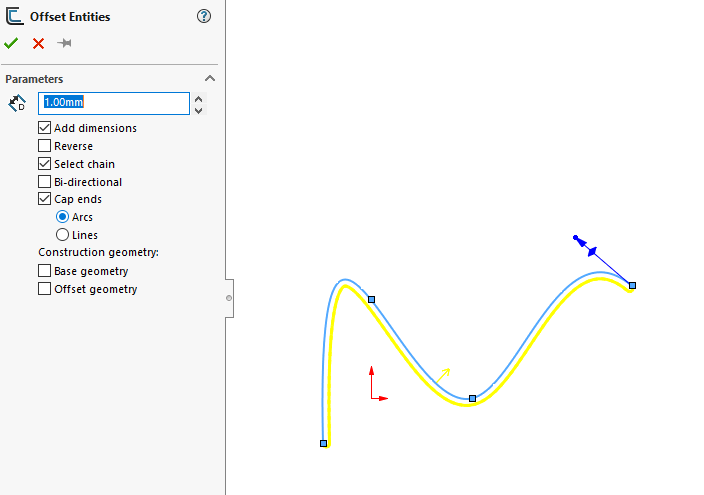
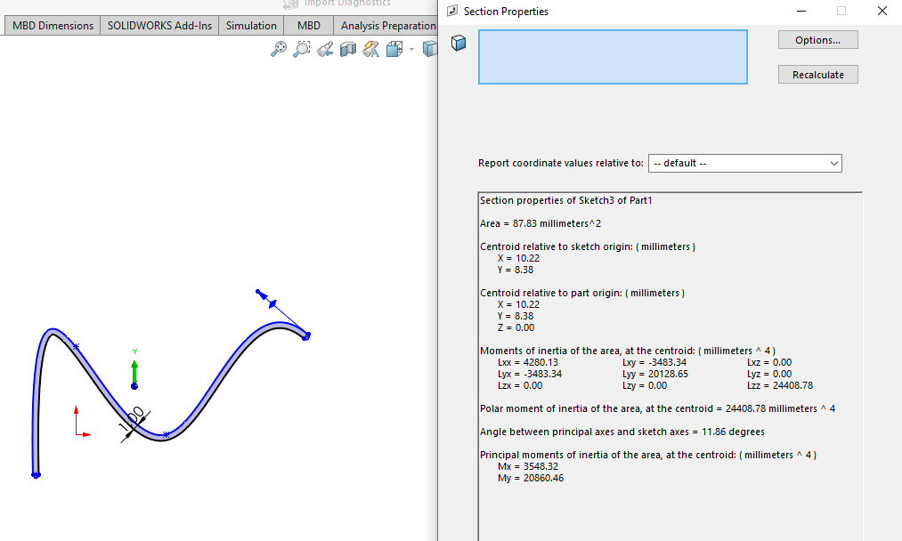
If we need to determine the center of a infinitely thin object we can draw it as a line and do a thin offset using the Offset Entities tool.
after which we can use the Section Properties tool to get the desired information.
Thus we can keep the discussion of center of mass to a minimum and skip computing countless examples of trivial cases for the sake of filling a course with material.
Center of mass by measuring
Center of mass – How CAD computes it
A CAD system stores a solid by its boundary. The model is a set of faces, each lying on a plane, a cylinder, a cone, a sphere, a torus or a spline surface and trimmed by its edges, and a STEP file carries exactly this description from one program to another. There is no interior to integrate over, so the volume integrals above must first be turned into integrals over the boundary. The divergence theorem does this. For a vector field \(\bm F\) in a volume \(V\) with the closed surface \(S\) and the outward unit normal \(\bm n\),
and we are free to choose any field whose divergence is the integrand we want. With \(\bm F = \bm r/3\) the divergence is one, and the left side is the volume,
\[
V = \frac{1}{3}\oint_S \bm r\cdot\bm n\,dA .
\tag{5.3.2}\]
We choose \(\bm F = \bm r/3\) without loss of generality. Any field with unit divergence gives the same volume, and \(\bm r/3\) is the one that treats the three directions alike. The result does not depend on the origin either: moving it by a constant vector \(\bm c\) adds \(\tfrac13\,\bm c\cdot\oint_S \bm n\,dA\), and the normals of a closed surface sum to zero. The surface must be closed, though, with the normals pointing outward, or the volume comes out wrong.
Code
%config InlineBackend.figure_formats = ['svg']import numpy as npimport sympy as spimport pandas as pdimport matplotlib.pyplot as pltimport build123d as bdfrom OCP.BRepTools import BRepToolsfrom OCP.BRepMesh import BRepMesh_IncrementalMeshfrom mechanicskit import ltxdef triangulate(shape, deflection):# build123d keeps an existing triangulation and reads the tolerance relative to the# edge lengths, so we remove the old triangles and ask OpenCascade for an absolute# deflection: no point of a triangle lies further than this from the true surface BRepTools.Clean_s(shape.wrapped) BRepMesh_IncrementalMesh(shape.wrapped, deflection, False, 0.5, True) verts, tris = shape.tessellate(deflection, 0.5)return np.array([[q.X, q.Y, q.Z] for q in verts]), np.array(tris)
NoteBut what is divergence?
Think of \(\bm F\) as the velocity of a fluid. The divergence \(\nabla\cdot\bm F\) at a point tells how much fluid is created there, per unit volume and unit time: how strongly the point acts as a source, or, where it is negative, as a sink. Multivariable calculus defines it as a sum of derivatives,
and a small box with the sides \(dx\), \(dy\) and \(dz\) shows why this sum measures an outflow. Through the face at \(x + dx\) the amount \(F_x(x + dx)\,dy\,dz\) flows out, through the face at \(x\) the amount \(F_x(x)\,dy\,dz\) flows in, and the net outflow is \(\partial F_x/\partial x\,dx\,dy\,dz\). The faces normal to \(y\) and \(z\) add the other two terms, so the divergence is the net outflow per unit volume,
\[
\nabla\cdot\bm F = \lim_{\Delta V \to 0}\frac{1}{\Delta V}\oint_{\partial(\Delta V)} \bm F\cdot\bm n\,dA .
\]
Now fill the body with such boxes and add up their outflows. Every inner face is shared by two boxes, and what leaves one box enters its neighbour, so the inner faces cancel and only the outer surface \(S\) remains. That sum is the divergence theorem, 5.3.1: what all the sources inside produce must leave through the surface.
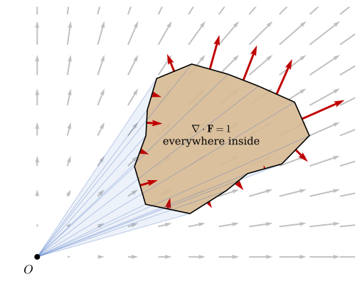
The field \(\bm F = \bm r/3\) is a flow that expands evenly in every direction, with \(\nabla\cdot\bm F = \tfrac13 + \tfrac13 + \tfrac13 = 1\). Every unit of volume produces one unit of outflow, so the total outflow through \(S\) equals the volume inside. The plane version is drawn below: \(\bm F = \bm r/2\) has unit divergence in two dimensions, the same argument gives the area \(A = \tfrac12\oint \bm r\cdot\bm n\,ds\), and for a polygon this becomes a sum of triangles with the origin, the shoelace formula that the 2D sketcher above uses for the trapezoid.
Code
# the region: a blob away from the origin, as a polygon with K verticesK =14phi = np.linspace(0, 2*np.pi, K, endpoint=False)rad =0.9+0.18*np.cos(3*phi) +0.1*np.sin(2*phi)poly = np.column_stack([2.3+1.2*rad*np.cos(phi), 1.6+ rad*np.sin(phi)])nxt = np.roll(poly, -1, axis=0)mid = (poly + nxt)/2edge = nxt - polyn_out = np.column_stack([edge[:, 1], -edge[:, 0]])/np.linalg.norm(edge, axis=1)[:, None] # counter-clockwise polygonA_shoelace =0.5*np.sum(poly[:, 0]*nxt[:, 1] - nxt[:, 0]*poly[:, 1])fig, ax = plt.subplots(figsize=(6, 4.4))gx, gy = np.meshgrid(np.linspace(0, 4, 11), np.linspace(0, 3.2, 9))ax.quiver(gx, gy, gx/2, gy/2, color='0.75', angles='xy', scale_units='xy', scale=4.5, width=0.004)for p, q inzip(poly, nxt): # the fan of triangles from O ax.fill([0, p[0], q[0]], [0, p[1], q[1]], color='#4472c4', alpha=0.05, lw=0) ax.plot([0, p[0]], [0, p[1]], color='#4472c4', lw=0.5, alpha=0.5)ax.fill(*poly.T, color='#d8ba94', alpha=0.9, lw=0)ax.plot(*np.vstack([poly, poly[:1]]).T, color='k', lw=1.2)Fn = np.einsum('ij,ij->i', mid/2, n_out) # F.n, the outflow per unit lengthax.quiver(mid[:, 0], mid[:, 1], Fn*n_out[:, 0], Fn*n_out[:, 1], color='#c00000', angles='xy', scale_units='xy', scale=3.2, width=0.006)ax.plot(0, 0, 'ko', ms=5); ax.text(-0.18, -0.22, r'$O$', fontsize=13)ax.text(2.3, 1.6, r'$\nabla\cdot\mathbf{F} = 1$'+'\neverywhere inside', ha='center', va='center', fontsize=11)ax.set_aspect('equal'); ax.set_xlim(-0.4, 4.2); ax.set_ylim(-0.4, 3.3); ax.set_axis_off()plt.tight_layout(); plt.show()
The field \(\bm F = \bm r/2\) in grey, a region in tan, and the flux \((\bm F\cdot\bm n)\,\bm n\) through its edges in red, pointing out where the flow leaves and in where it enters. The source strength is one everywhere inside, so the net outflow equals the area. Each edge and the origin \(O\) span a triangle, in blue, whose signed area is the edge’s share of the outflow. The triangles of the edges facing \(O\) count negative and cancel the part of the fan outside the region, the plane counterpart of the tetrahedra below. Grant Sanderson’s video Divergence and curl on 3Blue1Brown shows the fluid picture in motion.
The first moments follow from \(\bm F = \tfrac12 x^2\bm e_x\), whose divergence is \(x\), and the second moments from \(\bm F = \tfrac13 x^3\bm e_x\) and \(\bm F = \tfrac12 x^2 y\,\bm e_x\),
with the other components found by permuting \(x\), \(y\) and \(z\). Every quantity in this chapter, and the moments of inertia that rigid body kinetics needs, is therefore a surface integral. CAD software evaluates these integrals in one of two ways.
Exact faces and numerical quadrature
Each face is the image of a region in a parameter plane, \(\bm r(u, v)\), and the vector area element is \(\bm n\,dA = \bm r_{,u}\times\bm r_{,v}\,du\,dv\). 5.3.2 becomes a sum of double integrals over the parameter regions of the faces, which the software evaluates with Gauss quadrature on the exact geometry. OpenCascade, the geometry kernel of FreeCAD and of the Python library build123d that we use below, does this in its BRepGProp package. A cylinder of radius \(R\) and length \(L\) shows the bookkeeping. Its mantle is \(\bm r = [R\cos u,\ R\sin u,\ v]^\mathsf{T}\) with \(0 \le u \le 2\pi\) and \(0 \le v \le L\), and the two end disks are plane, with \(\bm r\cdot\bm n = L\) on the top and \(\bm r\cdot\bm n = 0\) on the bottom.
Code
R, L, u, v = sp.symbols('R L u v', positive=True)rr = sp.Matrix([R*sp.cos(u), R*sp.sin(u), v])nA = rr.diff(u).cross(rr.diff(v)) # n dA per du dv, pointing out of the cylinderV_mantle = sp.integrate(sp.simplify(rr.dot(nA))/3, (u, 0, 2*sp.pi), (v, 0, L))V_top = L*sp.pi*R**2/3# r.n = L over the disk areaV_bottom =0# r.n = 0, the disk passes through the originV_cyl = sp.simplify(V_mantle + V_top + V_bottom)
On the mantle \(\bm r\cdot(\bm r_{,u}\times\bm r_{,v}) = R^2\), and the three faces contribute
\[ \begin{aligned}V_\text{mantle} &= \dfrac{2 \pi L R^{2}}{3}\\ V_\text{top} &= \dfrac{\pi L R^{2}}{3}\\ V_\text{bottom} &= 0\\ V &= \pi L R^{2}\end{aligned} \]
which is the familiar volume of the cylinder. A spline face has no closed form for these integrals, and the quadrature then decides the accuracy.
Flat triangles
For display, for simulation and for 3D printing, the faces are instead replaced by triangles that lie within a chosen deflection \(\delta\) of the true surface, and an STL file contains nothing else. On a flat triangle with the vertices \(\bm a\), \(\bm b\) and \(\bm c\), numbered counter-clockwise seen from outside, the normal is constant and every point has the same \(\bm r\cdot\bm n = \bm a\cdot\bm n\). The triangle’s share of 5.3.2 is then
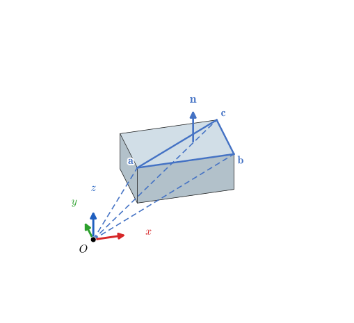
the signed volume of the tetrahedron with the triangle as base and the origin as apex, Figure 5.3.1. It is positive where the triangle faces away from the origin and negative where it faces the origin, so the sum over all triangles adds and removes tetrahedra until exactly the solid remains. This is the composite table of the previous section once more, with tetrahedra as the parts and the negative volumes in the role of the holes.
Figure 5.3.1: The top face of a box split into two triangles. The blue triangle with the vertices \(\bm a\), \(\bm b\) and \(\bm c\) and the outward normal \(\bm n\) spans a tetrahedron with the origin \(O\), and the signed volume of that tetrahedron is the triangle’s share of the surface integral for the volume.
The centroid of tetrahedron \(k\) is the mean of its four vertices, \((\bm a + \bm b + \bm c)/4\), since the fourth vertex is the origin. For the second moments we map the unit tetrahedron onto it, \(\bm r = \xi\bm a + \eta\bm b + \zeta\bm c\) with \(\xi, \eta, \zeta \ge 0\) and \(\xi + \eta + \zeta \le 1\), so that \(dV = 6V_k\,d\xi\,d\eta\,d\zeta\). Every integral then reduces to one of four integrals over the unit tetrahedron.
Code
xi, eta, zeta = sp.symbols('xi eta zeta', nonnegative=True)def over_unit_tet(f):return sp.integrate(f, (zeta, 0, 1- xi - eta), (eta, 0, 1- xi), (xi, 0, 1))I_1, I_xi, I_xixi, I_xieta = (over_unit_tet(f) for f in (1, xi, xi**2, xi*eta))
By symmetry the same values hold for \(\eta\) and \(\zeta\), and integrating over the unit tetrahedron gives
Moved to the centre of mass, \(\bm S_C = \bm S - V\bar{\bm r}\bar{\bm r}^\mathsf{T}\), and for a body of density \(\rho\) the inertia tensor about the centre of mass is
The integrals over each tetrahedron are exact, so the only error is in the geometry: the triangles cut across the curved faces as chords, and the results converge to the exact values as the deflection \(\delta\) goes to zero.
Example 1: A bracket from a STEP file
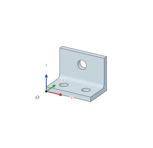
The steel bracket in Figure 5.3.2 has a base plate of \(80 \cdot 50 \cdot 8\) mm, an upright of \(80 \cdot 8 \cdot 58\) mm, a fillet of radius 6 mm in the inner corner, two holes of diameter 14 mm in the base and one of diameter 16 mm in the upright. It is stored in the file bracket.step, with the outer corner at the origin. Determine the mass, the centre of mass and the inertia tensor about the centre of mass from a triangulation of the file, with \(\rho = 7850\) kg/m³, and compare them with the exact values from the CAD kernel.
Figure 5.3.2: The steel bracket of Example 1, read from bracket.step, with the outer corner at the origin \(O\).
We read the file with build123d and let OpenCascade triangulate it with a deflection of \(\delta = 0.01\) mm, which the helper triangulate in the first code cell of this section does. The sums of 5.3.5 then take a few lines of NumPy, one row per triangle.
Code
rho =7850e-9# kg/mm^3bracket = bd.import_step("models/bracket.step")def mass_properties(P, T): a, b, c = P[T[:, 0]], P[T[:, 1]], P[T[:, 2]] V_k = np.einsum('ij,ij->i', a, np.cross(b, c))/6# signed tetrahedron volumes V = V_k.sum() rr_C = (V_k[:, None]*(a + b + c)/4).sum(axis=0)/V S =sum(np.einsum('k,ki,kj->ij', V_k, q, q) for q in (a, b, c, a + b + c))/20 S_C = S - V*np.outer(rr_C, rr_C)return V, rr_C, S_CP, T = triangulate(bracket, 0.01)V, rr_C, S_C = mass_properties(P, T)m = rho*VJ_C = rho*(np.trace(S_C)*np.eye(3) - S_C) # kg mm^2
The triangulation has 1140 triangles, and the sums give the volume, the mass and the centre of mass
\[ V = 60552.5\ \text{mm}^3,\quad m = 0.4753\ \text{kg},\quad \bar{\bm r} = \left[\begin{matrix}40.0\\35.904\\18.478\end{matrix}\right]\ \text{mm} \]
The bracket is symmetric about the plane \(x = 40\) mm, so its centre of mass lies in that plane, and the same symmetry makes \(J_{xy}\) and \(J_{xz}\) vanish. The inertia tensor about the centre of mass is
OpenCascade’s own integration over the exact faces, the BRepGProp route of the previous section, gives the reference values. Build123d returns them as volume, center() and matrix_of_inertia, the last one for unit density.
Side by side, the two routes agree to within about \(10^{-4}\):
triangles, δ = 0.01 mm
exact faces
relative difference
quantity
V (mm³)
60552.5
60546.5
+9.8e-05
m (kg)
0.475337
0.47529
+9.8e-05
x̄ (mm)
40
40
+2.7e-15
ȳ (mm)
35.904
35.9043
-6.4e-06
z̄ (mm)
18.4779
18.4783
-2.4e-05
Jxx (kg mm²)
253.339
253.323
+6.3e-05
Jyy (kg mm²)
412.933
412.906
+6.6e-05
Jzz (kg mm²)
365.165
365.14
+6.6e-05
Jyz (kg mm²)
-69.3438
-69.3381
-8.2e-05
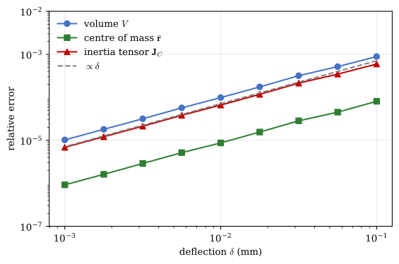
The triangulated volume is slightly too large. The chords of the holes and of the fillet cut through the concave surfaces on the side of the air, so the triangles remove a little less material than the exact model does. Figure 5.3.3 repeats the computation for deflections from 0.1 mm down to 0.001 mm. The relative errors fall in proportion to \(\delta\), along the line of slope one in the logarithmic plot, so halving the deflection halves the error, and the exact result is the limit of the triangulated one.
Figure 5.3.3: Relative error of the triangulated volume, centre of mass and inertia tensor of the bracket against the exact values from OpenCascade, as the deflection of the triangulation is reduced. All three errors are proportional to the deflection.
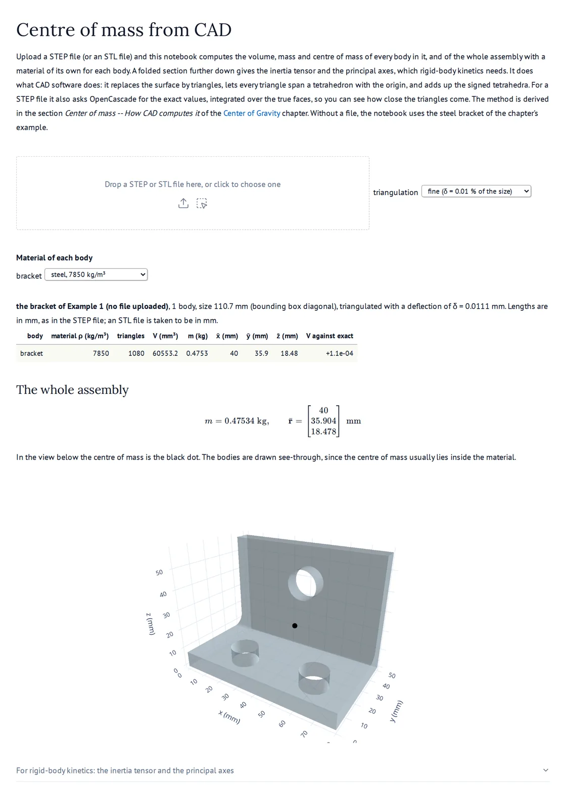
To do the same with your own models, open the marimo notebook Centre of mass from CAD in a new tab, Figure 5.3.4. It reads a STEP or STL file you upload, lists the volume, mass and centre of mass of every body in it with a material of its own, and compares the triangulated values with the exact ones. A folded section gives the inertia tensor and the principal axes of the assembly, which we return to in rigid body kinetics. The notebook runs on the book’s server and needs nothing installed. To run it on your own computer instead, install the packages with uv pip install marimo build123d plotly and open it with marimo edit CentroidFromCAD.py.
Figure 5.3.4: The marimo notebook Centre of mass from CAD with the bracket of Example 1. Click the picture to open the live notebook in a new tab, then drop your own STEP file on it.