8.17 Plasticity
A control arm that has hit a kerb too hard comes back bent. The load is gone, the arm carries almost no stress, and still it does not return to its original shape. Every chapter so far has used a material that springs back, Hooke’s law 8.6.1 in one dimension and 8.9.7 in three. This chapter is about the deformation that stays.
Plasticity matters to an engineer for two reasons. A ductile part that is overloaded deforms visibly before it breaks, and that deformation absorbs energy, the purpose of a bumper or a crash box. And a finite element model of such a part needs a material model that knows the material yields, since a linear model reports stresses far above the yield strength without complaint, as The linear assumptions in Chapter 8.20 discusses. Anyone who reads an FE result in which something yields has to know what the plasticity model in the solver assumes.
We first look inside metals, polymers and foams to see what elastic and plastic deformation are physically. We then return to the tensile test to split the strain into an elastic and a plastic part, and build three simple one-dimensional models from it. The yield criteria of Chapter 8.10 then become a three-dimensional model through a flow rule and a hardening rule, and the chapter closes with the algorithm that every FE solver runs at every point of every element in every step, the return mapping.
What elastic means
Elastic deformation is deformation the material gives back. Pull a steel bar to half its yield strength and let go, and it returns to its original length along the line it came up, with no trace of the load. The reason differs from one class of material to the next, and so does the size of the modulus.
In a metal the atoms sit at an equilibrium spacing \(r_0\) where the attraction and repulsion between neighbours balance. Pulled apart by a small distance, two atoms resist with a force proportional to the stretch, so each bond acts as a linear spring whose stiffness is the slope \(dF/dr\) of the force-distance curve at \(r_0\). A lattice of such springs gives a Young’s modulus of the order of that slope divided by \(r_0\). The atoms keep their neighbours while the lattice stretches, and when the load goes, every bond returns to \(r_0\). This also explains why all steels have \(E \approx 210~\text{GPa}\) while their yield strengths differ by a factor of ten: alloying and heat treatment change how easily the lattice slips, but hardly the bonds themselves.
A polymer is a tangle of long chains, held together along each chain by covalent bonds and between chains by much weaker van der Waals forces and entanglements. Below the glass transition temperature \(T_g\) the chains are frozen in place, and a load stretches bonds and pushes chains against their neighbours. The polymer is glassy, with \(E \approx 3~\text{GPa}\). Above \(T_g\) the chain segments rotate freely and the chains uncoil under load. The resistance now comes from the chains’ tendency to return to a coiled shape, the polymer is rubbery, and its modulus drops to \(1\) to \(10~\text{MPa}\). Rubber is elastic to strains of several hundred percent, but not linearly, and is described by a strain energy density \(W(\varepsilon)\) with \(\sigma = dW/d\varepsilon\), a hyperelastic material. PLA has its glass transition near \(60~^\circ\text{C}\), so a printed PLA part left in a car on a summer day can soften enough to sag under its own weight.
A foam is a network of thin cell walls, and under load the walls bend. Bending is a soft mode of deformation, so a foam is far less stiff than the material it is made of. For open-cell foams the modulus scales with the square of the relative density [1],
\[ \frac{E^*}{E_s} \approx \left(\frac{\rho^*}{\rho_s}\right)^2 \]
where \(E^*\) and \(\rho^*\) belong to the foam and \(E_s\) and \(\rho_s\) to the solid wall material. A foam of a tenth of the density has a hundredth of the stiffness. An elastomeric foam compressed further has its walls buckle, and still springs back when unloaded.
A fibre composite puts stiff fibres in a soft matrix. Along the fibres the stiffness \(E_1\) is set mainly by the fibres, across them \(E_2\) mainly by the matrix, and at the angle \(\theta\) to the fibres the modulus of a unidirectional ply is
\[ \frac{1}{E(\theta)} = \frac{\cos^4\theta}{E_1} + \left(\frac{1}{G_{12}} - \frac{2\nu_{12}}{E_1}\right)\sin^2\theta\cos^2\theta + \frac{\sin^4\theta}{E_2} \]
with the in-plane shear modulus \(G_{12}\) and Poisson’s ratio \(\nu_{12}\). A carbon-epoxy ply with \(E_1 = 140~\text{GPa}\), \(E_2 = 10~\text{GPa}\), \(G_{12} = 5~\text{GPa}\) and \(\nu_{12} = 0.3\) has \(E(45^\circ) = 13~\text{GPa}\), barely more than across the fibres: off the fibre direction, the soft matrix carries the load in shear. Hooke’s law then needs a full stiffness matrix \(\bm D\) with different moduli in different directions, the anisotropy that printed parts show across their layers, It is not isotropic.
In one dimension all of this reduces to a spring, Figure 8.17.1 (a). A spring is rate independent: it gives the same stress at the same strain however fast it is loaded. Polymers are not, and the simplest model that captures it adds a damper of viscosity \(\eta\), whose stress is proportional to its rate of extension. In panel (b), the standard linear solid, a spring \(E_\infty\) is parallel to a spring \(E_1\) in series with the damper. The stress \(\sigma_1\) in the damper branch relaxes with the time constant \(\tau = \eta/E_1\),
\[ \sigma = E_\infty\varepsilon + \sigma_1, \qquad \dot\sigma_1 + \frac{\sigma_1}{\tau} = E_1\dot\varepsilon \]
so a load applied much faster than \(\tau\) meets the stiffness \(E_\infty + E_1\), since the damper has no time to move, while a load applied much slower meets only \(E_\infty\). The stiffness depends on the rate, the material is viscoelastic, and it is still elastic in the sense that it returns to its original shape once it has had time to relax.
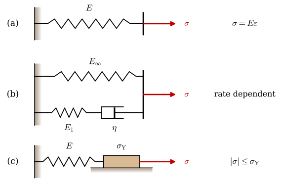
Panel (c) adds the element this chapter is about. A friction slider stays put until the force on it reaches a threshold and then slides at whatever rate the load demands. In series with a spring it gives a material that is elastic up to the stress \(\sigma_\text{Y}\) and flows at that stress beyond it. When the load is removed, the spring springs back and the slider stays where it slid to.
Why materials yield
Yielding is the start of deformation that stays. In metals it happens because dislocations glide, in polymers because chains slide past each other, and in foams because cell walls buckle, yield or break. The mechanisms are different, and a single continuum framework with different yield functions describes all three.
Dislocations in metals
Shearing a perfect crystal would mean sliding one plane of atoms over the next, which requires breaking every bond across the plane at the same time. The estimate for that stress is of the order of \(G/10\), several gigapascal for steel. Real crystals of pure metals start to slip at shear stresses thousands of times lower. Taylor, Orowan and Polanyi explained the gap independently in 1934 [2]: crystals contain dislocations, lines along which the lattice is out of register.
Figure 8.17.2 (a) shows an edge dislocation, an extra half plane of atoms ending at the slip plane. Under a shear stress \(\tau\) the bonds at the end of the half plane switch partners one row at a time, so the dislocation moves along the slip plane while only a few bonds are stretched at once. When it leaves the crystal, the upper half has moved by one atomic spacing over the lower half. A plastic strain we can see is the sum of an enormous number of such steps. Before and after each step the lattice is perfect, so the volume of the crystal does not change: plastic flow of a metal conserves volume.
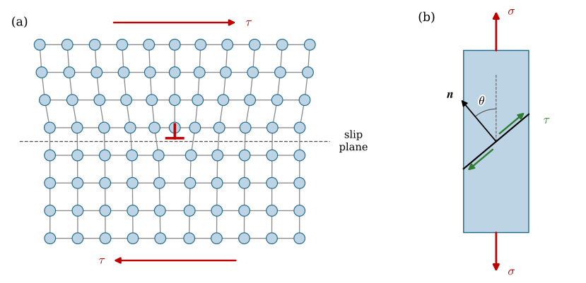
Only shear moves a dislocation. In the bar of panel (b) the traction on a plane whose normal makes the angle \(\theta\) with the axis has the normal component \(\sigma\cos^2\theta\) and the shear component
\[ \tau = \sigma\cos\theta\sin\theta = \frac{\sigma}{2}\sin 2\theta \tag{8.17.1}\]
which is largest, \(\sigma/2\), on planes at \(45^\circ\) to the axis. Slip starts when this resolved shear stress on a slip plane reaches a critical value \(\tau_c\) of the crystal, Schmid’s law [3]. In a real crystal the slip planes and slip directions are fixed by the lattice, and in a polycrystal they point every way, so some grain always has a plane close to \(45^\circ\). A hydrostatic pressure gives no shear on any plane, and so it moves no dislocations. This is why the yield criteria of Chapter 8.10 depend on the deviatoric stress alone, and why a metal does not yield under hydrostatic pressure however large.
Grain boundaries and hardening
A metal part is a polycrystal. As the melt solidifies, crystals grow from many nuclei until they meet, and each grain is a crystal with its own orientation. A dislocation gliding through one grain cannot pass straight into the next, since the slip planes do not line up, so dislocations pile up against the grain boundary. A pile-up concentrates stress at its head, and slip carries on in the next grain once that stress is large enough. Smaller grains hold shorter pile-ups, which concentrate less stress, so a finer-grained metal needs a larger applied stress to yield. The Hall-Petch relation [4,5]
\[ \sigma_\text{Y} = \sigma_0 + \frac{k}{\sqrt{d}} \tag{8.17.2}\]
gives the yield stress in terms of the grain size \(d\), with the lattice friction stress \(\sigma_0\) and a material constant \(k\). Halving the grain size raises the second term by \(41~\%\). Controlled rolling and cooling to refine the grains is how structural steels gain strength without expensive alloying.
As the plastic strain grows, sources inside the grains emit dislocation after dislocation, and their density rises by orders of magnitude. They tangle and block each other’s paths, so each further step of slip needs a higher stress. This is strain hardening, or work hardening. A paper clip bent once is harder to bend back at the same place, and bent back and forth it hardens until it breaks. In the continuum model, hardening appears as a yield stress that grows with the accumulated plastic strain.
Polymers and foams
A polymer has no lattice to slip. It yields when the stress becomes large enough for chain segments to rotate and chains to slide past each other, a process helped along by temperature and by time, so the yield stress of a polymer depends strongly on temperature and strain rate. A compressive pressure packs the chains tighter and makes sliding harder, and polymers therefore yield at a higher stress in compression than in tension.
A tensile specimen of a ductile polymer such as polyethylene shows this most clearly. After yield a neck forms, as in a metal. In the neck the chains straighten and align with the load, which makes the necked material much stiffer and stronger, so the neck stops thinning. It grows along the specimen instead, drawing material in from the shoulders at an almost constant force, until the whole gauge length has been drawn. This cold drawing reaches strains of several hundred percent. A metal neck, in contrast, keeps thinning until it breaks.
A foam compressed beyond its elastic range collapses by elastic buckling of the walls in an elastomeric foam, by plastic hinges in the walls of a metal or rigid polymer foam, or by fracture of the walls in a brittle one. The collapse starts in the weakest layer of cells and spreads layer by layer at an almost constant stress, the plateau stress. Once every cell has collapsed, the walls touch and the stress rises steeply, the stage called densification [1]. The plateau is why foams are used to absorb energy at a bounded force, in helmets, packaging and bumper absorbers. A foam also collapses under a hydrostatic pressure, since the cells can be crushed from all sides at once, so unlike a metal it yields without any deviatoric stress at all.
Rolled sheet
Rolling stretches the grains of a sheet and turns their crystal axes towards preferred directions, a texture, so the plastic properties of a rolled sheet depend on the direction. The usual measure is the r-value or Lankford coefficient. A tensile strip is cut from the sheet at an angle to the rolling direction, stretched past yield, and its plastic strains in the width and the thickness are measured,
\[ r = \frac{\varepsilon^p_w}{\varepsilon^p_t} \]
A material that yields equally in every direction has \(r = 1\), since the volume is conserved and the width and thickness then shrink by the same plastic strain. A sheet with \(r > 1\) resists thinning, as deep drawing needs, and \(r\) measured at \(0^\circ\), \(45^\circ\) and \(90^\circ\) to the rolling direction is what anisotropic yield criteria such as Hill’s [6] are fitted to. The rest of this chapter treats isotropic materials.
Elastic, plastic and true strain
The additive split
Load a tensile specimen of a metal past yield and then unload it. The unloading curve is a straight line parallel to the initial elastic line, with slope \(E\): on unloading the bonds relax while the dislocations stay where they have moved to. At zero stress a strain remains, the plastic strain \(\varepsilon^p\), and the part recovered on unloading, \(\sigma/E\), is the elastic strain \(\varepsilon^e\). The total strain is their sum,
\[ \varepsilon = \varepsilon^e + \varepsilon^p \tag{8.17.3}\]
and Hooke’s law holds for the elastic part only,
\[ \sigma = E\varepsilon^e = E\left(\varepsilon - \varepsilon^p\right) \tag{8.17.4}\]
The plastic strain is the record of the material’s history. Reloaded, the specimen is elastic up to the stress at which it was unloaded and yields only there: it remembers how far it was loaded. A plasticity model is a rule for how \(\varepsilon^p\) evolves; 8.17.4 then gives the stress. The additive split assumes small strains. Metal forming and crash simulations with large strains split the deformation multiplicatively instead, a refinement that changes the bookkeeping but not the ideas of this chapter [7].
Stored and dissipated energy
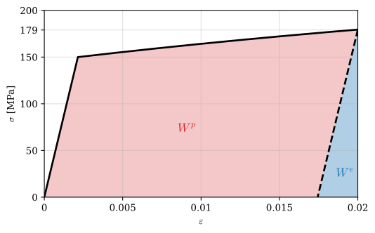
The work done on a unit volume of the specimen is the area under its stress-strain curve, \(W = \int\sigma\,d\varepsilon\). On unloading from the stress \(\sigma\), the triangle under the unloading line,
\[ W^e = \frac{\sigma^2}{2E} \tag{8.17.5}\]
comes back as work. The rest, \(W^p = W - W^e\), is dissipated: dislocations moving through the lattice turn it into heat. Taylor and Quinney compared the heat given off by metal bars twisted to large strains with the work done on them and found that around \(90~\%\) of the plastic work becomes heat, the rest staying stored in the dislocation structure [8]. Figure 8.17.3 shows the two areas for an aluminium alloy loaded to a strain of \(2~\%\).
Code
E_al, sy0_al, Q_al, b_al = 70e3, 150.0, 100.0, 20.0     # MPa, illustrative aluminium alloy
sigma_y_voce = lambda ep: sy0_al + Q_al*(1 - np.exp(-b_al*ep))
eps_end = 0.02
ep_end = brentq(lambda ep: sigma_y_voce(ep)/E_al + ep - eps_end, 0, eps_end)
s_end = sigma_y_voce(ep_end)

ep = np.linspace(0, ep_end, 200)
eps_load = np.r_[0, sigma_y_voce(ep)/E_al + ep]
sig_load = np.r_[0, sigma_y_voce(ep)]

fig, ax = plt.subplots(figsize=(6, 3.6))
ax.fill_between(eps_load, sig_load, color='C3', alpha=0.25, lw=0)
ax.fill_between([ep_end, eps_end], [0, s_end], color='white', lw=0)
ax.fill_between([ep_end, eps_end], [0, s_end], color='C0', alpha=0.35, lw=0)
ax.plot(eps_load, sig_load, color='black', lw=2)
ax.plot([eps_end, ep_end], [s_end, 0], color='black', lw=2, ls='--')
ax.text(0.0085, 70, '$W^p$', fontsize=13, color='C3')
ax.text(0.0186, 22, '$W^e$', fontsize=13, color='C0')
ax.set_xlabel(r'$\varepsilon$')
ax.set_ylabel(r'$\sigma$ [MPa]')
ax.set_xticks([0, 0.005, 0.01, 0.015, 0.02], ['0', '0.005', '0.01', '0.015', '0.02'])
ax.set_yticks([0, 50, 100, 150, round(s_end), 200])
ax.set_xlim(0, 0.02)
ax.set_ylim(0, 200)
ax.grid(True, alpha=0.4)
plt.show()The elastic triangle is a small part of the whole, and it becomes smaller the further the material is loaded. A spring can only store energy and give it back, while plastic deformation keeps it. This is the reason crash structures are made of ductile metals and foams that deform plastically: the kinetic energy of the car goes into plastic work and does not come back as a rebound.
Engineering and true stress
The tensile test of Chapter 8.6 reports the engineering stress and strain of 8.6.3, the force over the original area and the elongation over the original length. Both describe the specimen well while it is elastic, when its area and length change by a fraction of a percent. Plastic strains are a hundred times larger, and the area shrinks with them. Since plastic flow conserves volume, a result we prove from the flow rule below, \(AL = A_0L_0\) in the gauge length, and the true stress, the force over the current area, is
\[ \sigma_t = \frac{F}{A} = \frac{F}{A_0}\frac{L}{L_0} = \sigma(1 + \varepsilon) \]
The true strain adds up the increments of length relative to the current length,
\[ \varepsilon_t = \int_{L_0}^{L}\frac{dL}{L} = \ln\frac{L}{L_0} = \ln(1 + \varepsilon) \tag{8.17.6}\]
For small strains the two measures agree, and at \(\varepsilon = 0.2\) the true strain is \(0.18\). True strains of successive stretches add up, which engineering strains do not.
These relations hold while the deformation is uniform along the gauge length, and they stop holding when the specimen starts to neck. Necking begins at the largest force, where \(dF = 0\). With \(F = \sigma_t A\) and, from the constant volume, \(dA/A = -dL/L = -d\varepsilon_t\), that condition reads
\[ dF = A\,d\sigma_t + \sigma_t\,dA = 0 \quad\Rightarrow\quad \frac{d\sigma_t}{d\varepsilon_t} = \sigma_t \tag{8.17.7}\]
the criterion of Considère: the neck forms when the hardening of the material can no longer make up for the loss of area. For a material that hardens as a power law, \(\sigma_t = K\varepsilon_t^n\), the criterion gives the true strain at necking directly. Writing the engineering stress as \(\sigma = \sigma_t/(1 + \varepsilon) = K\varepsilon_t^n e^{-\varepsilon_t}\) and setting its derivative to zero must give the same result.
Code
K, n, eps_t = sp.symbols('K n varepsilon_t', positive=True)
sigma_true = K*eps_t**n
sigma_eng = sigma_true*sp.exp(-eps_t)                          # sigma_t/(1 + eps), eps = e^eps_t - 1

considere = sp.solve(sp.Eq(sp.diff(sigma_true, eps_t), sigma_true), eps_t)   # @eq-plasticity-considere
peak_eng = sp.solve(sp.diff(sigma_eng, eps_t), eps_t)

ltx(r"\frac{d\sigma_t}{d\varepsilon_t} = \sigma_t &\Rightarrow \varepsilon_t =", considere[0],
    r"\\ \frac{d\sigma}{d\varepsilon_t} = 0 &\Rightarrow \varepsilon_t =", peak_eng[0], aligned=True)
\[ \begin{aligned}\frac{d\sigma_t}{d\varepsilon_t} = \sigma_t &\Rightarrow \varepsilon_t =n\\ \frac{d\sigma}{d\varepsilon_t} = 0 &\Rightarrow \varepsilon_t =n\end{aligned} \]
Both conditions give \(\varepsilon_t = n\): for a power-law material the strain at the largest force equals the hardening exponent. Figure 8.17.4 draws both curves for \(K = 600~\text{MPa}\) and \(n = 0.21\), values chosen for illustration.
Code
K_h, n_h = 600.0, 0.21
et = np.linspace(1e-4, 0.4, 400)
st = K_h*et**n_h
e_eng = np.exp(et) - 1
s_eng = st/(1 + e_eng)
e_neck = np.exp(n_h) - 1

fig, ax = plt.subplots(figsize=(6, 3.6))
ax.plot(et, st, color='C3', lw=2, label=r'true, $\sigma_t$ against $\varepsilon_t$')
ax.plot(e_eng, s_eng, color='C0', lw=2, label=r'engineering, $\sigma$ against $\varepsilon$')
ax.plot(e_neck, K_h*n_h**n_h*np.exp(-n_h), 'o', color='C0', ms=6)
ax.axvline(e_neck, color='0.35', lw=0.8, ls=':')
ax.text(e_neck + 0.008, 120, r'necking, $\varepsilon_t = n$', fontsize=10)
ax.set_xlabel('strain')
ax.set_ylabel('stress [MPa]')
ax.set_xticks([0, 0.1, e_neck, 0.4, 0.49], ['0', '0.1', f'{e_neck:.3f}', '0.4', '0.49'])
ax.set_yticks([0, 100, 200, 300, 400, 500])
ax.set_xlim(0, 0.49)
ax.set_ylim(0, 500)
ax.grid(True, alpha=0.4)
ax.legend(loc='lower right')
plt.show()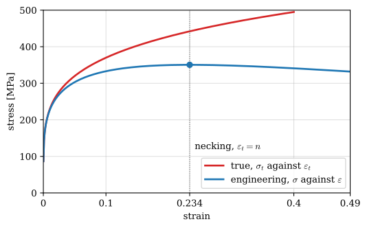
This matters directly for finite element input. LS-DYNA and most other codes expect the hardening curve as true stress against the plastic part of the true strain, \(\varepsilon^p = \varepsilon_t - \sigma_t/E\). A curve typed in as engineering stress against engineering strain understates the stress at large strains, and the measured curve ends at necking, so the part of the curve beyond it has to be extrapolated or calibrated against a simulation of the test.
Three common models
A plasticity model needs the yield stress as a function of how much the material has flowed. In one dimension the measure is the accumulated plastic strain, which in monotonic tension is \(\varepsilon^p\) itself; in three dimensions it becomes the effective plastic strain \(\varepsilon^p_{\text{eff}}\), defined below. The slope of the yield stress against this strain is the plastic modulus,
\[ E_p = \frac{d\sigma_\text{Y}}{d\varepsilon^p_{\text{eff}}} \]
Three models cover most engineering use, Figure 8.17.5. The elastic, perfectly plastic model has \(E_p = 0\) and a constant yield stress. This is the friction slider of Figure 8.17.1 (c). It ignores hardening and gives the limit loads of steel structures. The linear hardening model has a constant plastic modulus,
\[ \sigma_\text{Y} = \sigma_{\text{Y}0} + E_p\,\varepsilon^p_{\text{eff}} \tag{8.17.8}\]
and the nonlinear hardening model takes \(\sigma_\text{Y}(\varepsilon^p_{\text{eff}})\) from a measured curve or a fitted law, e.g. \(\sigma_\text{Y} = \sigma_{\text{Y}0} + Q\left(1 - e^{-\beta\varepsilon^p_{\text{eff}}}\right)\), which saturates at \(\sigma_{\text{Y}0} + Q\). Each can be given a fracture strain \(\varepsilon_f\), the effective plastic strain at which the material is taken to fail. It is the simplest failure criterion there is, and the one behind the eroding elements discussed later.
In tension beyond yield, the linear hardening model has a straight line of slope smaller than \(E\). Its strain is the elastic part 8.17.4 plus the plastic part from 8.17.8, \(\varepsilon = \sigma/E + (\sigma - \sigma_{\text{Y}0})/E_p\), so
\[ \frac{d\sigma}{d\varepsilon} = E_t = \frac{EE_p}{E + E_p} \tag{8.17.9}\]
the tangent modulus: the elastic and plastic compliances add like two springs in series. LS-DYNA’s *MAT_PIECEWISE_LINEAR_PLASTICITY asks for \(E_t\) (the field ETAN) and converts it with \(E_p = EE_t/(E - E_t)\); since \(E_t\) is usually a percent or two of \(E\), the two differ little. The right panel of Figure 8.17.5 unloads and reloads the linear hardening model. Unloading follows the slope \(E\), reloading retraces the unloading line, and the material yields again at the stress where it was unloaded: its yield stress has grown to that value.
Code
E_s, sy0_s, Ep_s = 210e3, 250.0, 2100.0                  # MPa
eps_f = 0.1
models = {
    r'perfectly plastic, $E_p = 0$': lambda ep: sy0_s + 0*ep,
    r'linear, $E_p$ constant': lambda ep: sy0_s + Ep_s*ep,
    r'nonlinear, $E_p(\varepsilon^p_{\mathrm{eff}})$': lambda ep: sy0_s + 200*(1 - np.exp(-30*ep)),
}

fig, (ax1, ax2) = plt.subplots(1, 2, figsize=(9.5, 3.6))
for (name, sy), c in zip(models.items(), ('C3', 'C1', 'C2')):
    ep_f = brentq(lambda ep: sy(ep)/E_s + ep - eps_f, 0, eps_f)
    ep = np.linspace(0, ep_f, 200)
    ax1.plot(np.r_[0, sy(ep)/E_s + ep], np.r_[0, sy(ep)], color=c, lw=2, label=name)
    ax1.plot(eps_f, sy(ep_f), 'x', color=c, ms=9, mew=2)
ax1.axvline(eps_f, color='0.35', lw=0.8, ls=':')
ax1.text(eps_f - 0.011, 160, r'$\varepsilon_f$', fontsize=12)
ax1.set_xlabel(r'$\varepsilon$')
ax1.set_ylabel(r'$\sigma$ [MPa]')
ax1.set_xticks([0, 0.04, 0.08, 0.1, 0.12], ['0', '0.04', '0.08', '0.1', '0.12'])
ax1.set_yticks([0, 100, 250, 400, 500])
ax1.set_xlim(0, 0.12)
ax1.set_ylim(0, 500)
ax1.grid(True, alpha=0.4)
ax1.legend(fontsize=9, loc='lower right')

# load to 3 %, unload to zero stress, reload to 6 %: linear hardening
Et_s = E_s*Ep_s/(E_s + Ep_s)                             # @eq-plasticity-tangent
ey = sy0_s/E_s
s1 = sy0_s + Et_s*(0.03 - ey)
ep1 = 0.03 - s1/E_s
s2 = s1 + Et_s*(0.06 - 0.03)
ax2.plot([0, ey, 0.03], [0, sy0_s, s1], color='C1', lw=2, label='loading')
ax2.plot([0.03, ep1], [s1, 0], color='C0', lw=2, ls='--', label='unloading and reloading')
ax2.plot([0.03, 0.06], [s1, s2], color='C1', lw=2)
ax2.axhline(s1, color='0.35', lw=0.8, ls=':')
ax2.text(0.002, s1 + 6, r'new yield stress', fontsize=10)
ax2.set_xlabel(r'$\varepsilon$')
ax2.set_ylabel(r'$\sigma$ [MPa]')
ax2.set_xticks([0, 0.015, 0.03, 0.045, 0.06], ['0', '0.015', '0.03', '0.045', '0.06'])
ax2.text(ep1 - 0.0065, 15, r'$\varepsilon^p$', fontsize=12, color='C0')
ax2.set_yticks([0, 100, 200, 250, round(s1), 380])
ax2.set_xlim(0, 0.06)
ax2.set_ylim(0, 380)
ax2.grid(True, alpha=0.4)
ax2.legend(fontsize=9, loc='lower right')
fig.tight_layout()
plt.show()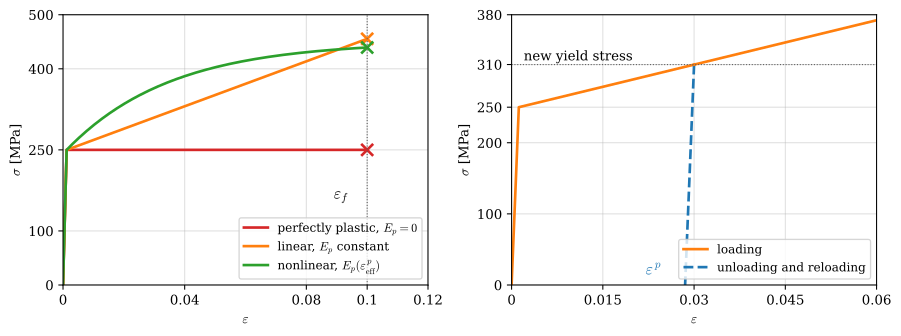
Example 1: A bar loaded past yield
A steel bar of length \(L_0 = 200~\text{mm}\) and cross-sectional area \(A = 50~\text{mm}^2\) is fixed at one end, Figure 8.17.6 (a). Its other end is pulled out by \(u = 2~\text{mm}\) and then released. The steel follows the linear hardening model of panel (b) with \(E = 210~\text{GPa}\), \(\sigma_{\text{Y}0} = 250~\text{MPa}\) and \(E_p = 2.1~\text{GPa}\). Determine the largest force, the permanent elongation after release, the new yield stress, and how the work done on the bar divides into stored and dissipated energy.
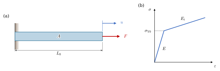
The stress is uniform along the bar, so the bar is a tensile specimen and the one-dimensional model applies directly. The strain is \(\varepsilon = u/L_0\) and the strain at first yield \(\varepsilon_\text{Y} = \sigma_{\text{Y}0}/E\). If \(\varepsilon > \varepsilon_\text{Y}\), the stress follows from 8.17.9 and the force from the area,
\[ \sigma = \sigma_{\text{Y}0} + E_t\left(\varepsilon - \varepsilon_\text{Y}\right), \qquad F = \sigma A \]
The plastic strain is what remains of the strain when the elastic part is removed, 8.17.4. Releasing the bar unloads it along the slope \(E\) to zero stress, so the plastic strain stays as the permanent strain, and by 8.17.8 the new yield stress is
\[ \varepsilon^p = \varepsilon - \frac{\sigma}{E}, \qquad \Delta L_p = \varepsilon^p L_0, \qquad \sigma_\text{Y} = \sigma_{\text{Y}0} + E_p\varepsilon^p \]
The work per unit volume is the area under the two straight pieces of the loading curve, the stored part is 8.17.5, and each is multiplied by the volume \(V = AL_0\),
\[ W = \frac{\sigma_{\text{Y}0}\varepsilon_\text{Y}}{2} + \frac{(\sigma_{\text{Y}0} + \sigma)(\varepsilon - \varepsilon_\text{Y})}{2}, \qquad W^e = \frac{\sigma^2}{2E}, \qquad W^p = W - W^e \]
If all of the dissipated work turns into heat and none of it leaves the bar, the steel, with density \(\rho = 7850~\text{kg/m}^3\) and specific heat \(c = 460~\text{J/(kg K)}\), warms by \(\Delta T = W^p/(\rho V c)\).
L_0, A_b, u_b = 200.0, 50.0, 2.0                      # mm, mm^2, mm
E, sigma_y0, E_p = 210e3, 250.0, 2100.0               # MPa
E_t = E*E_p/(E + E_p)                                 # @eq-plasticity-tangent

eps = u_b/L_0
eps_y = sigma_y0/E
sigma = sigma_y0 + E_t*(eps - eps_y)                  # eps > eps_y, so the bar has yielded
F = sigma*A_b                                         # N

eps_p = eps - sigma/E                                 # what is left after unloading along E
dL_p = eps_p*L_0
sigma_y_new = sigma_y0 + E_p*eps_p                    # @eq-plasticity-linear-hardening

V = A_b*L_0                                           # mm^3; MPa mm^3 = mJ
W = (sigma_y0*eps_y/2 + (sigma_y0 + sigma)*(eps - eps_y)/2)*V/1e3     # J
W_e = sigma**2/(2*E)*V/1e3
W_p = W - W_e
dT = W_p/(7850*V*1e-9*460)                            # K, with V in m^3

ltx(r"F_{\max} &=", F/1e3, r"~\text{kN}, \quad \varepsilon^p =", eps_p,
    r", \quad \Delta L_p =", dL_p, r"~\text{mm}, \quad \sigma_\text{Y} =", sigma_y_new, r"~\text{MPa}",
    r"\\ W &=", W, r"~\text{J}, \quad W^e =", W_e, r"~\text{J}, \quad W^p =", W_p,
    r"~\text{J}, \quad \Delta T =", dT, r"~\text{K}", aligned=True, precision=4)
\[ \begin{aligned}F_{\max} &=13.42~\text{kN}, \quad \varepsilon^p =0.008722, \quad \Delta L_p =1.744~\text{mm}, \quad \sigma_\text{Y} =268.3~\text{MPa}\\ W &=24.32~\text{J}, \quad W^e =1.714~\text{J}, \quad W^p =22.6~\text{J}, \quad \Delta T =0.626~\text{K}\end{aligned} \]
The largest force is \(13.4~\text{kN}\) at the stress \(268~\text{MPa}\). Of the \(2~\text{mm}\) the end was pulled out, \(1.74~\text{mm}\) remains, and the springback \(\sigma L_0/E = 0.26~\text{mm}\) is the elastic part. The yield stress has risen from \(250\) to \(268~\text{MPa}\), the stress at which the bar was released, and a second pull will be elastic up to that stress. Of the \(24.3~\text{J}\) of work, \(93~\%\) is dissipated and only \(1.7~\text{J}\) comes back on release. The temperature rise of \(0.6~\text{K}\) is small, but it grows in proportion to the plastic strain, and in a crash, where strains reach tens of percent in milliseconds, the heated zones of a steel structure get tens of kelvin warmer. Figure 8.17.7 draws the load path with the two energies.
Code
fig, ax = plt.subplots(figsize=(6, 3.6))
ax.fill_between([0, eps_y, eps, eps_p], [0, sigma_y0, sigma, 0], color='C3', alpha=0.25, lw=0)
ax.fill_between([eps_p, eps], [0, sigma], color='C0', alpha=0.35, lw=0)
ax.plot([0, eps_y, eps], [0, sigma_y0, sigma], color='black', lw=2)
ax.plot([eps, eps_p], [sigma, 0], color='black', lw=2, ls='--')
ax.plot(eps_p, 0, 'o', color='black', ms=6)
ax.text(0.0035, 100, rf'$W^p = {W_p:.1f}$ J', fontsize=11, color='C3')
ax.text(eps_p + 0.0005, 30, r'$W^e$', fontsize=12, color='C0')
ax.set_xlabel(r'$\varepsilon$')
ax.set_ylabel(r'$\sigma$ [MPa]')
ax.set_xticks([0, round(eps_y, 5), 0.004, round(eps_p, 5), 0.01])
ax.set_xticklabels(['0', rf'{eps_y:.4f}', '0.004', rf'{eps_p:.4f}', '0.01'])
ax.set_yticks([0, 100, 200, 250, round(sigma), 300])
ax.set_xlim(0, 0.0105)
ax.set_ylim(0, 300)
ax.grid(True, alpha=0.4)
plt.show()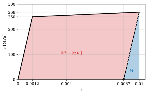
Continuum plasticity
The bar of Example 1 has one stress. A point in a control arm has six, the components of the stress tensor 8.7.6, and a three-dimensional model needs the same ingredients as the bar in tensor form: the strain split into an elastic and a plastic part, an elastic law, a condition that says when the material yields, a rule for the direction in which it then flows, and a rule for how the yield stress grows. Chapter 8.10 supplied the condition. In this section it becomes a model.
The yield function
The yield criterion 8.10.1 compares an effective stress with the yield strength. For a material that hardens, the yield strength becomes the current yield stress \(\sigma_\text{Y}(\varepsilon^p_{\text{eff}})\), a function of how much the material has flowed, and the criterion becomes a yield function,
\[ \phi(\bm\sigma, \varepsilon^p_{\text{eff}}) = \sigma_\text{vM}(\bm\sigma) - \sigma_\text{Y}(\varepsilon^p_{\text{eff}}) \tag{8.17.10}\]
with the von Mises stress written through the deviator, 8.10.12,
\[ \sigma_\text{vM} = \sqrt{\tfrac{3}{2}\,\bm s : \bm s} \]
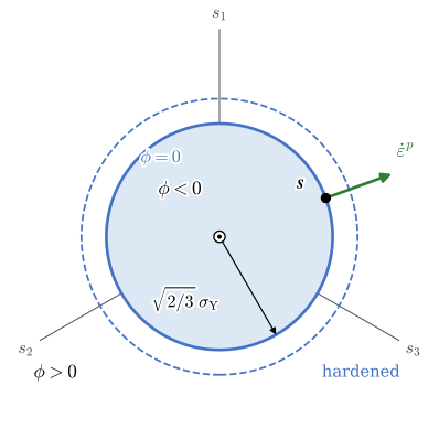
where \(\bm s = \bm\sigma - \sigma_m\bm I\) is the stress deviator 8.10.7, \(\sigma_m\) the mean stress 8.10.6, and \(\bm s : \bm s = s_{ij}s_{ij}\) the sum of the squares of all nine components. The value of \(\phi\) sorts every stress state into one of three cases. With \(\phi < 0\) the material is elastic. With \(\phi = 0\) the stress is on the yield surface and the material may flow. A state with \(\phi > 0\) is not allowed: the model never lets the stress go there, and when a computation produces one, the solver has to correct it, the subject of the last section.
In principal stress space, the Haigh–Westergaard space of Chapter 8.10, the surface \(\phi = 0\) is a cylinder around the hydrostatic axis \(\sigma_1 = \sigma_2 = \sigma_3\), as Chapter 8.10 showed. Looking down that axis, the cylinder is the circle of Figure 8.17.8 in the deviatoric plane. Each stress state projects to its deviatoric part \(\bm s\) in that plane, while its hydrostatic part moves it along the axis, out of the page, without changing \(\phi\). From 8.10.12 the length of \(\bm s\) is \(\sqrt{\bm s : \bm s} = \sqrt{2/3}\,\sigma_\text{vM}\), so the circle has the radius \(\sqrt{2/3}\,\sigma_\text{Y}\).
The flow rule
When the material flows, the yield function also fixes the direction of the plastic strain rate. The associated flow rule makes it normal to the yield surface,
\[ \dot{\bm\varepsilon}^p = \dot\lambda\,\frac{\partial\phi}{\partial\bm\sigma} = \dot\lambda\,\bm n, \qquad \bm n = \frac{3}{2}\frac{\bm s}{\sigma_\text{vM}} \tag{8.17.11}\]
where the plastic multiplier \(\dot\lambda \geq 0\) sets how fast the material flows and \(\bm n\) in which direction. The normal follows from differentiating \(\sigma_\text{vM}^2 = \frac{3}{2}\bm s : \bm s\). Since \(\bm s : \bm I = 0\), a change of the mean stress does not change \(\bm s : \bm s\), so \(2\sigma_\text{vM}\,d\sigma_\text{vM} = 3\,\bm s : d\bm s = 3\,\bm s : d\bm\sigma\), and \(\partial\sigma_\text{vM}/\partial\bm\sigma = 3\bm s/(2\sigma_\text{vM})\). For metals the normality rule agrees with measurements, and it gives the model a structure that is convenient to compute with.
Two consequences follow at once. The direction \(\bm n\) is deviatoric, \(\operatorname{tr}\bm n = 0\), so the plastic strain rate has no trace and the plastic part of the volumetric strain 8.9.9 stays zero: plastic flow conserves volume, the continuum version of the perfect lattice before and after a dislocation has passed. And in uniaxial tension, \(\bm\sigma = \operatorname{diag}(\sigma, 0, 0)\), the direction is \(\bm n = \operatorname{diag}(1, -\frac{1}{2}, -\frac{1}{2})\): the lateral plastic strain is minus half the axial one, the plastic strain behaves as if Poisson’s ratio were \(\frac{1}{2}\). The total Poisson’s ratio of a specimen therefore moves from its elastic value towards \(\frac{1}{2}\) as the plastic strain grows.
The amount of plastic flow is measured by the effective plastic strain, which accumulates the magnitude of the plastic strain rate,
\[ \varepsilon^p_{\text{eff}} = \int_0^t\dot\varepsilon^p_{\text{eff}}\,dt, \qquad \dot\varepsilon^p_{\text{eff}} = \sqrt{\tfrac{2}{3}\,\dot{\bm\varepsilon}^p : \dot{\bm\varepsilon}^p} \tag{8.17.12}\]
The factor \(\frac{2}{3}\) is chosen so that in uniaxial tension \(\varepsilon^p_{\text{eff}}\) equals the axial plastic strain. It never decreases, whichever way the material flows. FE post-processors plot it as “effective plastic strain”, and failure criteria compare it with \(\varepsilon_f\). Inserting 8.17.11 shows that \(\dot\varepsilon^p_{\text{eff}} = \dot\lambda\), so the plastic multiplier is the rate of effective plastic strain. We check the uniaxial case.
Code
sig = sp.symbols('sigma', positive=True)
lam_dot = sp.symbols(r'\dot{\lambda}', positive=True)

S = sp.diag(sig, 0, 0)
s = S - S.trace()/3*sp.eye(3)                                   # @eq-stress-deviator
sigma_bar = sp.sqrt(sp.Rational(3, 2)*sum(s[i, j]**2 for i in range(3) for j in range(3)))
n_dir = sp.simplify(sp.Rational(3, 2)*s/sigma_bar)              # @eq-plasticity-flow-rule
deps_p = lam_dot*n_dir
deps_eff = sp.sqrt(sp.Rational(2, 3)*sum(deps_p[i, j]**2 for i in range(3) for j in range(3)))

ltx(r"\sigma_\text{vM} &=", sigma_bar, r", \qquad \bm n =", n_dir,
    r"\\ \operatorname{tr}\bm n &=", n_dir.trace(), r", \qquad \dot\varepsilon^p_{\text{eff}} =",
    sp.simplify(deps_eff), aligned=True)
\[ \begin{aligned}\sigma_\text{vM} &=\sigma, \qquad \bm n =\left[\begin{matrix}1 & 0 & 0\\0 & - \dfrac{1}{2} & 0\\0 & 0 & - \dfrac{1}{2}\end{matrix}\right]\\ \operatorname{tr}\bm n &=0, \qquad \dot\varepsilon^p_{\text{eff}} =\dot{\lambda}\end{aligned} \]
Hardening
With isotropic hardening the yield surface grows uniformly with the effective plastic strain, and the circle of Figure 8.17.8 widens to the dashed one. The linear version is 8.17.8 with \(\varepsilon^p_{\text{eff}}\) from 8.17.12, and the nonlinear version takes \(\sigma_\text{Y}(\varepsilon^p_{\text{eff}})\) from a curve of true stress against plastic strain. Isotropic hardening grows the surface the same amount in every direction, so a bar stretched until it yields at \(300~\text{MPa}\) will yield in compression at \(-300~\text{MPa}\). Real metals reverse earlier, the Bauschinger effect, because the dislocation pile-ups that resist forward slip help reverse slip along. Kinematic hardening models this by moving the surface in the direction of flow without growing it. The difference matters under cyclic loading and for springback after forming; for loads that increase monotonically, isotropic hardening is the standard choice. LS-DYNA’s *MAT_PLASTIC_KINEMATIC mixes the two through a parameter \(\beta\), from purely kinematic at \(\beta = 0\) to purely isotropic at \(\beta = 1\).
Loading and unloading
Plastic flow happens only on the yield surface. The three conditions
\[ \dot\lambda \geq 0, \qquad \phi \leq 0, \qquad \dot\lambda\,\phi = 0 \tag{8.17.13}\]
say this in one line: either the stress is inside the surface and the material is elastic, \(\phi < 0\) and \(\dot\lambda = 0\), or it flows, \(\dot\lambda > 0\), and then it must be on the surface, \(\phi = 0\). While it flows, the stress stays on the growing surface, so \(\dot\phi = 0\), the consistency condition, which fixes \(\dot\lambda\). A stress on the surface that moves inwards, \(\dot\phi < 0\), is unloading: \(\dot\lambda = 0\), and the response is elastic. This is why the tensile specimen unloads along the slope \(E\).
In one dimension the consistency condition reproduces the tangent modulus. With \(\phi = |\sigma| - \sigma_\text{Y}\) and tension, \(\dot\phi = \dot\sigma - E_p\dot\lambda = 0\), while 8.17.4 gives \(\dot\sigma = E(\dot\varepsilon - \dot\lambda)\). Eliminating \(\dot\sigma\) gives \(\dot\lambda = E\dot\varepsilon/(E + E_p)\) and \(\dot\sigma = EE_p\dot\varepsilon/(E + E_p)\), 8.17.9 once more.
The model in equations
Collected, the model for a von Mises material with linear isotropic hardening reads
\[ \boxed{ \begin{aligned} \bm\varepsilon &= \bm\varepsilon^e + \bm\varepsilon^p \\ \bm\sigma &= \bm D\bm\varepsilon^e \\ \phi &= \sigma_\text{vM}(\bm\sigma) - \sigma_\text{Y}(\varepsilon^p_{\text{eff}}) \\ \dot{\bm\varepsilon}^p &= \dot\lambda\,\frac{3}{2}\frac{\bm s}{\sigma_\text{vM}}, \qquad \dot\varepsilon^p_{\text{eff}} = \dot\lambda \\ \sigma_\text{Y} &= \sigma_{\text{Y}0} + E_p\,\varepsilon^p_{\text{eff}} \\ \dot\lambda &\geq 0, \qquad \phi \leq 0, \qquad \dot\lambda\,\phi = 0 \end{aligned} } \tag{8.17.14}\]
where \(\bm D\) is the elastic stiffness of 8.9.7, applied to the elastic strain only. The first two rows are elasticity with the plastic strain subtracted, the third is the yield criterion, the fourth the flow rule, the fifth the hardening rule, and the last row decides between loading and unloading. The material parameters are \(E\), \(\nu\), \(\sigma_{\text{Y}0}\) and \(E_p\), or a hardening curve in place of the last two, and a fracture strain \(\varepsilon_f\) if the material is to fail. These are the fields of *MAT_PIECEWISE_LINEAR_PLASTICITY in LS-DYNA: E, PR, SIGY, ETAN or a curve, and FAIL.
Other yield surfaces, rate and damage
The von Mises cylinder describes metals, whose yielding does not depend on the pressure. Polymers, soils and concrete yield at a higher stress in compression than in tension, since pressure increases the friction between chains or grains. Their yield surfaces open up towards compression: the Drucker-Prager criterion is a cone around the hydrostatic axis [9], the Mohr-Coulomb criterion a pyramid with a hexagonal section. Foams, soils and powders also yield under pure hydrostatic compression, when the cells collapse or the grains pack closer, so their yield surfaces are closed by a cap on the compression side. With such surfaces the normal of the flow rule has a hydrostatic component, and the material changes volume as it flows: a foam compacts. LS-DYNA’s crushable foam models, used for bumper absorbers, let the foam yield under hydrostatic compression in this way.
Viscoplasticity adds a dependence on the strain rate: the faster the loading, the higher the flow stress. Steels are noticeably stronger at crash rates than in a quasi-static test, and *MAT_PIECEWISE_LINEAR_PLASTICITY scales its yield stress with the Cowper-Symonds law through its parameters C and P, or with a table of hardening curves for different rates.
Damage describes the voids that nucleate at inclusions, grow with the plastic strain and finally link up into a crack. The material carries less load as they grow, and continuum damage mechanics represents this with a damage variable \(D\) between zero and one that reduces the stiffness to \((1 - D)E\) [10], the model met in The stiffness does not come back. When \(D\) reaches one, or in the simplest form when \(\varepsilon^p_{\text{eff}}\) reaches \(\varepsilon_f\), the material at that point has failed, and an explicit solver removes the element from the model. These eroding elements turn a row of failed elements into a crack. The approach needs judgement. The element’s mass and energy leave the model with it, and the crack can only follow element boundaries. Once a material softens, the strain concentrates in a single row of elements, so the strain at which that row fails depends on the element size: halving the elements lets the same overall deformation produce larger strains in the row that fails. A failure strain is therefore calibrated for a mesh size, and the result of a simulation with eroding elements has to be checked against a model with a different mesh before it is trusted.
Computational plasticity
A finite element program computes displacements, Chapter 8.20. From them it computes the strain at every integration point of every element, and the material model has to turn that strain into a stress. With plasticity the answer depends on the history, so the program loads the model in steps. At each step and each integration point the material routine receives the stress \(\bm\sigma_n\), the plastic strain \(\bm\varepsilon^p_n\) and the effective plastic strain \(\varepsilon^p_{\text{eff},n}\) from the end of the previous step, together with the strain increment \(\Delta\bm\varepsilon\) of the current step, and returns the same quantities at the end of the step. The model 8.17.14 is imposed at the end of the step, the backward Euler method applied to the flow rule. The routine is strain driven, and it is the only place in the solver that knows the material has yielded.
Return mapping in one dimension
The algorithm first assumes that the step is elastic. Freezing the plastic strain gives the trial stress
\[ \sigma^* = \sigma_n + E\,\Delta\varepsilon, \qquad \phi^* = |\sigma^*| - \sigma_{\text{Y},n} \tag{8.17.15}\]
where \(\sigma_{\text{Y},n} = \sigma_{\text{Y}0} + E_p\varepsilon^p_{\text{eff},n}\). If \(\phi^* \leq 0\), the trial stress is inside or on the yield surface, the guess was right, and the step is elastic. If \(\phi^* > 0\), the trial stress is outside, and a plastic increment \(\Delta\lambda\) in the direction of \(\operatorname{sign}\sigma^*\) has to bring it back. The plastic strain grows by \(\Delta\lambda\operatorname{sign}\sigma^*\), which reduces the stress by \(E\Delta\lambda\), and the yield stress grows by \(E_p\Delta\lambda\). The end state must lie on the surface,
\[ |\sigma_{n+1}| - \sigma_{\text{Y},n+1} = |\sigma^*| - E\Delta\lambda - \sigma_{\text{Y},n} - E_p\Delta\lambda = 0 \quad\Rightarrow\quad \Delta\lambda = \frac{\phi^*}{E + E_p} \tag{8.17.16}\]
and the state is updated with
\[ \begin{aligned} \sigma_{n+1} &= \sigma^* - E\Delta\lambda\operatorname{sign}\sigma^* \\ \varepsilon^p_{n+1} &= \varepsilon^p_n + \Delta\lambda\operatorname{sign}\sigma^* \\ \varepsilon^p_{\text{eff},n+1} &= \varepsilon^p_{\text{eff},n} + \Delta\lambda \end{aligned} \]
The step is called a return mapping: an elastic predictor followed by a plastic corrector back to the yield surface. For linear hardening it is exact whatever the size of the step. The routine also returns the slope of the stress against the strain increment, \(E\) for an elastic step and \(E_t\) of 8.17.9 for a plastic one, which an implicit solver needs for its tangent stiffness.
def return_map_1d(sigma_n, eps_p_n, eps_peff_n, d_eps, E, sigma_y0, E_p):
    """One strain increment of the 1D elastic-plastic model with linear isotropic hardening.

    Returns the stress, plastic strain and effective plastic strain at the end of the
    step, and the tangent d sigma / d eps that an implicit solver assembles.
    """
    sigma_trial = sigma_n + E*d_eps                       # elastic predictor
    sigma_y_n = sigma_y0 + E_p*eps_peff_n
    phi_trial = abs(sigma_trial) - sigma_y_n
    if phi_trial <= 0:                                    # inside the surface: the step is elastic
        return sigma_trial, eps_p_n, eps_peff_n, E

    d_lam = phi_trial/(E + E_p)                           # @eq-plasticity-return-1d
    sign = np.sign(sigma_trial)
    sigma = sigma_trial - E*d_lam*sign                    # plastic corrector, back to the surface
    return sigma, eps_p_n + d_lam*sign, eps_peff_n + d_lam, E*E_p/(E + E_p)
We drive the routine through a strain history that pulls the material to \(\varepsilon = 0.01\), pushes it to \(-0.01\), and repeats once, in steps of \(10^{-4}\), with the steel of Example 1. The first peak must reproduce the stress and plastic strain found there by hand.
legs = [0, 0.01, -0.01, 0.01, -0.01, 0]
eps_hist = np.concatenate([np.linspace(a, b, int(round(abs(b - a)/1e-4)) + 1)[1:]
                           for a, b in zip(legs[:-1], legs[1:])])
eps_hist = np.r_[0, eps_hist]

state = (0.0, 0.0, 0.0)                                   # sigma, eps_p, eps_peff
hist = [state]
for k in range(1, len(eps_hist)):
    sigma_k, eps_p_k, eps_peff_k, _ = return_map_1d(*state, eps_hist[k] - eps_hist[k - 1],
                                                    E, sigma_y0, E_p)
    state = (sigma_k, eps_p_k, eps_peff_k)
    hist.append(state)
hist = np.array(hist)

i_peak = 100                                              # eps = 0.01, the end of the first leg
ltx(r"\sigma(\varepsilon = 0.01) &=", hist[i_peak, 0], r"~\text{MPa}, \quad \varepsilon^p =",
    hist[i_peak, 1], r"\\ \text{Example 1:}\ \sigma &=", sigma, r"~\text{MPa}, \quad \varepsilon^p =",
    eps_p, aligned=True, precision=5)
\[ \begin{aligned}\sigma(\varepsilon = 0.01) &=268.32~\text{MPa}, \quad \varepsilon^p =0.0087223\\ \text{Example 1:}\ \sigma &=268.32~\text{MPa}, \quad \varepsilon^p =0.0087223\end{aligned} \]
The routine agrees with Example 1 to all printed digits, as it should for linear hardening. Figure 8.17.9 shows the whole history.
Code
fig, (ax1, ax2) = plt.subplots(1, 2, figsize=(9.5, 3.6))
ax1.plot(eps_hist, hist[:, 0], color='C0', lw=2)
ax1.plot(eps_hist[0], 0, 'o', color='black', ms=5)
ax1.axhline(0, color='0.35', lw=0.8)
ax1.axvline(0, color='0.35', lw=0.8)
ax1.set_xlabel(r'$\varepsilon$')
ax1.set_ylabel(r'$\sigma$ [MPa]')
smax = np.ceil(np.abs(hist[:, 0]).max())
ax1.set_xticks([-0.01, -0.005, 0, 0.005, 0.01], ['−0.01', '−0.005', '0', '0.005', '0.01'])
ax1.set_yticks([-smax, -250, 0, 250, smax])
ax1.set_xlim(-0.01, 0.01)
ax1.set_ylim(-smax, smax)
ax1.grid(True, alpha=0.4)

steps = np.arange(len(eps_hist))
ax2.plot(steps, hist[:, 1], color='C1', lw=2, label=r'$\varepsilon^p$')
ax2.plot(steps, hist[:, 2], color='C2', lw=2, label=r'$\varepsilon^p_{\mathrm{eff}}$')
ax2.set_xlabel('step')
ax2.set_ylabel('plastic strain')
pmax = hist[:, 2].max()
ax2.set_xticks([0, 100, 300, 500, 700, steps[-1]])
pmin = hist[:, 1].min()
ax2.set_yticks([pmin, 0, 0.02, 0.04, pmax], [f'{pmin:.4f}'.replace('-', '−'), '0', '0.02', '0.04', f'{pmax:.4f}'])
ax2.set_xlim(0, steps[-1])
ax2.set_ylim(hist[:, 1].min(), pmax)
ax2.grid(True, alpha=0.4)
ax2.legend(loc='upper left')
fig.tight_layout()
plt.show()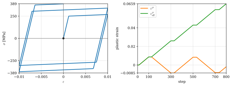
Every reversal unloads along the slope \(E\) and yields again at the current yield stress with the opposite sign. Isotropic hardening makes the loop grow with each half cycle. The area of a closed loop is the plastic work dissipated per cycle, and the effective plastic strain accumulates it without regard to sign. A failure criterion based on \(\varepsilon^p_{\text{eff}}\) therefore counts a small plastic strain cycled many times the same as a large one applied once, a crude model of low-cycle fatigue at best, Chapter 8.21.
Radial return in three dimensions
The three-dimensional algorithm has the same two steps. The elastic predictor uses Hooke’s law 8.9.7,
\[ \bm\sigma^* = \bm\sigma_n + \bm D\Delta\bm\varepsilon, \qquad \phi^* = \sigma^*_\text{vM} - \sigma_{\text{Y},n} \tag{8.17.17}\]
with \(\sigma^*_\text{vM}\) computed from the trial deviator \(\bm s^* = \bm\sigma^* - \sigma^*_m\bm I\) by 8.10.12. If \(\phi^* > 0\), the plastic corrector applies the flow rule 8.17.11 over the step, \(\Delta\bm\varepsilon^p = \Delta\lambda\,\frac{3}{2}\bm s_{n+1}/\sigma_{\text{vM},n+1}\). The plastic strain increment is deviatoric, so the mean stress does not change, \(\sigma_{m,n+1} = \sigma^*_m\). The deviator is reduced by the shear stiffness \(2G\) times the plastic strain increment,
\[ \bm s_{n+1} = \bm s^* - 2G\Delta\bm\varepsilon^p = \bm s^* - 3G\Delta\lambda\frac{\bm s_{n+1}}{\sigma_{\text{vM},n+1}} \]
The correction is parallel to \(\bm s_{n+1}\), so \(\bm s_{n+1}\) is parallel to \(\bm s^*\), and the stress returns along the radius of the circle, Figure 8.17.10. This radial return goes back to Wilkins’ hydrocodes of the 1960s [11]. Taking the effective stress of both sides gives \(\sigma_{\text{vM},n+1} = \sigma^*_\text{vM} - 3G\Delta\lambda\), and requiring the end state to lie on the hardened surface, \(\sigma_{\text{vM},n+1} = \sigma_{\text{Y},n} + E_p\Delta\lambda\), gives
\[ \Delta\lambda = \frac{\phi^*}{3G + E_p}, \qquad \bm s_{n+1} = \frac{\sigma_{\text{Y},n} + E_p\Delta\lambda}{\sigma^*_\text{vM}}\,\bm s^* \tag{8.17.18}\]
the one-dimensional 8.17.16 with \(E\) replaced by \(3G\). The difference comes from the lateral strains. In the bar, the plastic flow makes the cross section contract freely, while the strain increment given to the three-dimensional routine is prescribed in all directions, and the deviatoric stiffness \(2G\) acting on the flow direction \(\frac{3}{2}\bm s/\sigma_\text{vM}\) gives \(3G\).
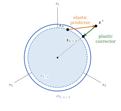
The routine below is the radial return that the LS-DYNA Theory Manual describes for its elastic-plastic materials with isotropic hardening, reduced to linear hardening and small strains [12].
nu = 0.3
G = E/(2*(1 + nu))
K_bulk = E/(3*(1 - 2*nu))
I3 = np.eye(3)

def radial_return(sigma_n, eps_p_n, eps_peff_n, d_eps, sigma_y0=sigma_y0, E_p=E_p):
    """One strain increment of von Mises plasticity with linear isotropic hardening.

    All tensors are 3x3 arrays. The elastic law is written with the bulk and shear moduli,
    which is @eq-generalized-hooke split into its mean and deviatoric parts.
    """
    d_mean = np.trace(d_eps)/3
    sigma_trial = sigma_n + 3*K_bulk*d_mean*I3 + 2*G*(d_eps - d_mean*I3)   # elastic predictor
    mean_trial = np.trace(sigma_trial)/3
    s_trial = sigma_trial - mean_trial*I3
    sbar_trial = np.sqrt(1.5*np.sum(s_trial*s_trial))                      # @eq-von-mises-deviator
    sigma_y_n = sigma_y0 + E_p*eps_peff_n
    phi_trial = sbar_trial - sigma_y_n
    if phi_trial <= 0:
        return sigma_trial, eps_p_n, eps_peff_n

    d_lam = phi_trial/(3*G + E_p)                                         # @eq-plasticity-return-3d
    s_new = (sigma_y_n + E_p*d_lam)/sbar_trial*s_trial                    # back along the radius
    eps_p = eps_p_n + d_lam*1.5*s_trial/sbar_trial                        # the flow rule over the step
    return s_new + mean_trial*I3, eps_p, eps_peff_n + d_lam
To compare it with the bar, the routine has to be run in uniaxial stress. Only the axial strain is prescribed, and in each step the lateral strain increment \(\Delta\varepsilon_{22} = \Delta\varepsilon_{33}\) is the one that leaves the lateral stress at zero,
\[ \sigma_{22}\left(\Delta\varepsilon_{22}\right) = 0 \]
a scalar equation that a root finder solves to machine precision. This is a small version of what a solver does for a whole model, where the equilibrium of every node decides the strains the material routine receives. The axial stress must then follow the 1D curve exactly, and the lateral plastic strain must be minus half the axial one.
def uniaxial_step(state, d_eps11):
    sigma_n, eps_p_n, eps_peff_n = state
    def lateral_stress(d_lat):
        d_eps = np.diag([d_eps11, d_lat, d_lat])
        return radial_return(sigma_n, eps_p_n, eps_peff_n, d_eps)[0][1, 1]
    d_lat = brentq(lateral_stress, -abs(d_eps11), abs(d_eps11), xtol=1e-16)
    return radial_return(sigma_n, eps_p_n, eps_peff_n, np.diag([d_eps11, d_lat, d_lat]))

state3 = (np.zeros((3, 3)), np.zeros((3, 3)), 0.0)
hist3 = [state3]
for k in range(1, len(eps_hist)):
    state3 = uniaxial_step(state3, eps_hist[k] - eps_hist[k - 1])
    hist3.append(state3)

sigma11 = np.array([h[0][0, 0] for h in hist3])
lateral = np.array([np.abs(h[0][1:, :]).max() for h in hist3])
ratio = hist3[i_peak][1][1, 1]/hist3[i_peak][1][0, 0]

ltx(r"\max_n\left|\sigma_{11} - \sigma_{\text{1D}}\right| &=", np.abs(sigma11 - hist[:, 0]).max(),
    r"~\text{MPa}, \quad \max_n|\sigma_{22}|, |\sigma_{33}|, |\tau| =", lateral.max(),
    r"~\text{MPa} \\ \varepsilon^p_{22}/\varepsilon^p_{11} &=", ratio,
    r", \quad \varepsilon^p_{\text{eff}} - |\varepsilon^p_{11}| \text{ at the first peak} =",
    hist3[i_peak][2] - abs(hist3[i_peak][1][0, 0]), aligned=True, precision=3)
\[ \begin{aligned}\max_n\left|\sigma_{11} - \sigma_{\text{1D}}\right| &=1.25 \cdot 10^{-12}~\text{MPa}, \quad \max_n|\sigma_{22}|, |\sigma_{33}|, |\tau| =1.26 \cdot 10^{-12}~\text{MPa} \\ \varepsilon^p_{22}/\varepsilon^p_{11} &=-0.5, \quad \varepsilon^p_{\text{eff}} - |\varepsilon^p_{11}| \text{ at the first peak} =0\end{aligned} \]
The three-dimensional radial return reproduces the 1D loop to round-off, the lateral stresses stay at zero, and the lateral plastic strain is minus half the axial, the plastic Poisson’s ratio of one half. In uniaxial stress, 8.17.18 and 8.17.16 describe the same material. Figure 8.17.11 overlays the two.
Code
fig, ax = plt.subplots(figsize=(6, 3.6))
ax.plot(eps_hist, hist[:, 0], color='C0', lw=4, alpha=0.4, label='1D return mapping')
ax.plot(eps_hist, sigma11, color='black', lw=1.2, ls='--', label=r'3D radial return, $\sigma_{11}$')
ax.set_xlabel(r'$\varepsilon_{11}$')
ax.set_ylabel(r'$\sigma_{11}$ [MPa]')
ax.set_xticks([-0.01, -0.005, 0, 0.005, 0.01], ['−0.01', '−0.005', '0', '0.005', '0.01'])
ax.set_yticks([-smax, -250, 0, 250, smax])
ax.set_xlim(-0.01, 0.01)
ax.set_ylim(-smax, smax)
ax.grid(True, alpha=0.4)
ax.legend(loc='upper center', bbox_to_anchor=(0.5, -0.2), ncol=2, fontsize=9)
plt.show()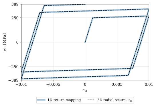
Explicit and implicit solvers
The finite element equations of motion are
\[ \bm M\ddot{\bm u} + \bm f_{\text{int}}(\bm u) = \bm f_{\text{ext}} \]
with the mass matrix \(\bm M\) and the internal forces \(\bm f_{\text{int}}\), which the solver assembles from the stresses the material routine returns. There are two ways to march this through time, and they differ by orders of magnitude in how often they call the material routine.
An explicit solver uses the central difference method with a diagonal (lumped) mass matrix. It computes the acceleration from the forces of the current step, \(\ddot{\bm u}_n = \bm M^{-1}\left(\bm f_{\text{ext}} - \bm f_{\text{int}}(\bm u_n)\right)\), and from it the displacements of the next step. No system of equations is solved, and each step calls the material routine once per integration point. The method is stable only while a stress wave crosses less than one element per step [13],
\[ \Delta t \leq \frac{L_e}{c}, \qquad c = \sqrt{\frac{E}{\rho}} \tag{8.17.19}\]
where \(L_e\) is the length of the smallest element and \(c\) the speed of sound in the material.
An implicit solver finds the equilibrium at the end of each step directly. For a static problem it solves \(\bm R(\bm u) = \bm f_{\text{ext}} - \bm f_{\text{int}}(\bm u) = \bm 0\) for the displacements with Newton’s method,
\[ \bm K_T\,\Delta\bm u = \bm R, \qquad \bm K_T = \frac{\partial\bm f_{\text{int}}}{\partial\bm u} \tag{8.17.20}\]
where the tangent stiffness \(\bm K_T\) is assembled from the tangents the material routine returns, \(E\) in elastic points and \(E_t\) in plastic ones in the 1D case. The steps can be large, but each one needs a few iterations, and each iteration factors a matrix with one row per degree of freedom. For a steel part meshed with \(5~\text{mm}\) elements, 8.17.19 gives the explicit time step and the number of steps a crash of \(100~\text{ms}\) takes.
Code
rho_s, L_e, t_end = 7850.0, 5e-3, 0.1                     # kg/m^3, m, s
c_s = np.sqrt(E*1e6/rho_s)                                # m/s, E in Pa
dt = L_e/c_s                                              # @eq-plasticity-time-step
n_steps = t_end/dt

ltx(r"c &=", c_s, r"~\text{m/s}, \quad \Delta t =", dt*1e6, r"~\mu\text{s}, \quad t/\Delta t =",
    n_steps/1e5, r"\cdot 10^5", aligned=True, precision=3)
\[ \begin{aligned}c &=5.17 \cdot 10^{3}~\text{m/s}, \quad \Delta t =0.967~\mu\text{s}, \quad t/\Delta t =1.03\cdot 10^5\end{aligned} \]
A microsecond per step and a hundred thousand steps, each calling the material routine at every integration point: a model with a million integration points makes about \(10^{11}\) calls. That is affordable only because each radial return costs a few dozen arithmetic operations. An implicit analysis of a slow load case takes perhaps fifty steps with a handful of iterations each, a few hundred calls per point, but solves a large linear system in every iteration. Explicit solvers are therefore used for short events with impact and contact, such as a crash or a drop test, and implicit solvers for slow loading and for static load cases. The explicit time step is set by the smallest element of the whole model: a single short element can slow an analysis down tenfold. LS-DYNA therefore lists the elements with the smallest time steps, and applies a safety factor of \(0.9\) to 8.17.19 by default. Mass scaling adds mass to the smallest elements to raise their time step, acceptable only as long as the added mass is a small fraction of the total and does not change the dynamics of the part.
Residual stress after a load cycle
A part loaded until some of it yields and then unloaded does not return to a stress-free state. The yielded material has been stretched permanently, the elastic material around it has not, and on unloading the elastic material pulls the yielded zone back and is held out by it. The part is left with residual stresses that balance each other without any load. At a hole in a plate loaded in tension past yield, the material at the edge of the hole is left in compression and the material further out in tension.
Since the unloading is elastic, the residual stresses follow from two solutions we already know how to compute: the stress at the peak load from the elastic-plastic model, minus the stress the same load would give in a purely elastic body,
\[ \bm\sigma_{\text{res}} = \bm\sigma(P) - \bm\sigma_{\text{el}}(P) \tag{8.17.21}\]
valid as long as the unloading does not itself cause yielding. Residual stresses can be put to use. A compressive residual stress at a notch lowers the mean stress of every later load cycle, Chapter 8.21, and that is why fastener holes in aircraft are cold expanded and pressure vessels and gun barrels are overloaded once on purpose, autofrettage. Welds leave residual stresses of the opposite, harmful sign, close to the yield strength, as the weld metal shrinks while it cools.
Example 2: Three bars loaded past yield and unloaded
A rigid beam hangs from three steel bars, Figure 8.17.12. The middle bar 1 has the length \(L_1 = 1.0~\text{m}\), the two outer bars 2 the length \(L_2 = 1.5~\text{m}\), and all three have the cross-sectional area \(A = 100~\text{mm}^2\). The steel is elastic, perfectly plastic with \(E = 210~\text{GPa}\) and \(\sigma_\text{Y} = 250~\text{MPa}\). A load \(P\) at the middle of the beam is raised to \(70~\text{kN}\) and removed. Determine the load at which the first bar yields, the bar forces and the displacement at \(70~\text{kN}\), and the residual stresses and the permanent displacement after unloading. At what load does the structure yield when it is loaded a second time?
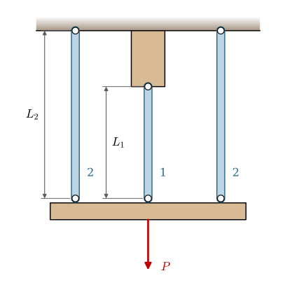
The structure is statically indeterminate, so the bar forces follow from equilibrium, compatibility and the material law together. By symmetry the beam moves down by \(u\) without turning, and the bars stretch by \(u\), so
\[ \varepsilon_1 = \frac{u}{L_1}, \qquad \varepsilon_2 = \frac{u}{L_2}, \qquad N_1 + 2N_2 = P \]
with \(N_i = \sigma_i A\) and \(\sigma_i = E(\varepsilon_i - \varepsilon^p_i)\), \(|\sigma_i| \leq \sigma_\text{Y}\). The short bar takes the larger strain and yields first. While all bars are elastic, \(P = EAu\left(1/L_1 + 2/L_2\right)\), and bar 1 reaches \(\sigma_\text{Y}\) at \(u_y = \sigma_\text{Y} L_1/E\), so the first yield load is
\[ P_\text{Y} = \sigma_\text{Y} A\left(1 + \frac{2L_1}{L_2}\right) \]
Beyond it, bar 1 carries the constant force \(\sigma_\text{Y} A\) and the outer bars take the rest elastically,
\[ N_1 = \sigma_\text{Y} A, \qquad N_2 = \frac{P - \sigma_\text{Y} A}{2}, \qquad u = \frac{N_2L_2}{EA} \]
until the outer bars also yield at the limit load \(P_L = 3\sigma_\text{Y} A\), where the structure can carry no more. Unloading from \(P\) to zero is elastic, so by 8.17.21 the changes are those of the elastic structure under \(-P\),
\[ \Delta u = -\frac{P}{EA\left(1/L_1 + 2/L_2\right)}, \qquad \Delta N_1 = \frac{EA\,\Delta u}{L_1}, \qquad \Delta N_2 = \frac{EA\,\Delta u}{L_2} \]
and the residual forces and displacement are the values at \(70~\text{kN}\) plus these changes.
A_3, L_1, L_2, sigma_y3 = 100.0, 1000.0, 1500.0, 250.0     # mm^2, mm, mm, MPa
P_max = 70e3                                               # N
EA = E*A_3

P_y = sigma_y3*A_3*(1 + 2*L_1/L_2)
P_L = 3*sigma_y3*A_3
N_1, N_2 = sigma_y3*A_3, (P_max - sigma_y3*A_3)/2         # bar 1 yielded, bars 2 elastic
u_max = N_2*L_2/EA

d_u = -P_max/(EA*(1/L_1 + 2/L_2))                         # elastic unloading
res_1 = (N_1 + EA*d_u/L_1)/A_3
res_2 = (N_2 + EA*d_u/L_2)/A_3
u_res = u_max + d_u

ltx(r"P_\text{Y} &=", P_y/1e3, r"~\text{kN}, \quad P_L =", P_L/1e3, r"~\text{kN}",
    r"\\ N_1 &=", N_1/1e3, r"~\text{kN}, \quad N_2 =", N_2/1e3, r"~\text{kN}, \quad u =", u_max, r"~\text{mm}",
    r"\\ \sigma_{1,\text{res}} &=", res_1, r"~\text{MPa}, \quad \sigma_{2,\text{res}} =", res_2,
    r"~\text{MPa}, \quad u_{\text{res}} =", u_res, r"~\text{mm}", aligned=True, precision=4)
\[ \begin{aligned}P_\text{Y} &=58.33~\text{kN}, \quad P_L =75.0~\text{kN}\\ N_1 &=25.0~\text{kN}, \quad N_2 =22.5~\text{kN}, \quad u =1.607~\text{mm}\\ \sigma_{1,\text{res}} &=-50.0~\text{MPa}, \quad \sigma_{2,\text{res}} =25.0~\text{MPa}, \quad u_{\text{res}} =0.1786~\text{mm}\end{aligned} \]
The middle bar yields at \(58.3~\text{kN}\), and at \(70~\text{kN}\) it carries \(25~\text{kN}\) and each outer bar \(22.5~\text{kN}\). After unloading, the middle bar is left in compression at \(-50~\text{MPa}\) and the outer bars in tension at \(25~\text{MPa}\); their forces, \(-5~\text{kN}\) and \(2 \cdot 2.5~\text{kN}\), balance with no load on the beam. The beam stays \(0.18~\text{mm}\) lower than before. Loaded a second time, bar 1 starts from \(-50~\text{MPa}\) and reaches \(+250~\text{MPa}\) only when the load has added \(300~\text{MPa}\) to it, which by the elastic solution happens at \(P = 70~\text{kN}\): the first overload has raised the load at which the structure yields from \(58.3\) to \(70~\text{kN}\). This is the principle of autofrettage on the smallest possible structure.
The same answer must come out of the computation an implicit FE solver makes. The beam’s displacement is the one unknown, and at each load step Newton’s method 8.17.20 drives the residual \(R(u) = P - A\left(\sigma_1 + 2\sigma_2\right)\) to zero, with the bar stresses from return_map_1d and the tangent stiffness assembled from the bar tangents,
\[ K_T = A\left(\frac{E_{t,1}}{L_1} + \frac{2E_{t,2}}{L_2}\right) \]
We load to \(70~\text{kN}\), unload to zero and load again to \(70~\text{kN}\), in steps of \(5~\text{kN}\). Since the material model is perfectly plastic, \(E_p = 0\), and the tangent of a yielded bar is zero.
P_hist = np.r_[np.linspace(0, P_max, 15), np.linspace(P_max, 0, 15)[1:], np.linspace(0, P_max, 15)[1:]]
lengths = np.array([L_1, L_2, L_2])                        # bar 1 and the two bars 2

u = 0.0
bars = [(0.0, 0.0, 0.0)]*3                                 # converged sigma, eps_p, eps_peff per bar
out = [(0.0, 0.0, 0.0, 0)]
for P in P_hist[1:]:
    u_n = u
    for it in range(20):
        trial = [return_map_1d(*bars[i], (u - u_n)/lengths[i], E, sigma_y3, 0.0) for i in range(3)]
        R = P - A_3*sum(t[0] for t in trial)               # out-of-balance force
        if abs(R) < 1e-6*P_max:
            break
        K_T = A_3*sum(t[3]/L for t, L in zip(trial, lengths))
        u = u + R/K_T                                      # @eq-plasticity-newton
    bars = [t[:3] for t in trial]                          # the step has converged: keep its state
    out.append((u, trial[0][0], trial[1][0], it))
out = np.array(out)

i_top, i_zero = 14, 28
ltx(r"\text{at } 70~\text{kN:}\ u &=", out[i_top, 0], r"~\text{mm}, \quad \sigma_1 =", out[i_top, 1],
    r"~\text{MPa}, \quad \sigma_2 =", out[i_top, 2], r"~\text{MPa}",
    r"\\ \text{unloaded:}\ u &=", out[i_zero, 0], r"~\text{mm}, \quad \sigma_1 =", out[i_zero, 1],
    r"~\text{MPa}, \quad \sigma_2 =", out[i_zero, 2], r"~\text{MPa}",
    r"\\ \text{Newton updates per step} &\leq", int(out[:, 3].max()), aligned=True, precision=4)
\[ \begin{aligned}\text{at } 70~\text{kN:}\ u &=1.607~\text{mm}, \quad \sigma_1 =250.0~\text{MPa}, \quad \sigma_2 =225.0~\text{MPa}\\ \text{unloaded:}\ u &=0.1786~\text{mm}, \quad \sigma_1 =-50.0~\text{MPa}, \quad \sigma_2 =25.0~\text{MPa}\\ \text{Newton updates per step} &\leq2\end{aligned} \]
The Newton solution agrees with the hand solution. Every elastic step converges after one update, since the model is linear there. The three steps from \(60\) to \(70~\text{kN}\) need two. The first of them crosses the yield load, and the other two start with bar 1 exactly on its yield surface, where the return mapping sees a zero strain increment for the first iterate, calls it elastic and returns the tangent \(E\). In all three the first update uses a tangent that is too stiff, the update falls short, bar 1 then flows and its tangent drops to zero, and the second update lands on the solution. With a piecewise linear model the tangent is exact once each bar is known to be elastic or plastic. Figure 8.17.13 shows the load path. On reloading the structure follows the unloading line all the way back to \(70~\text{kN}\), elastic throughout.
Code
fig, (ax1, ax2) = plt.subplots(1, 2, figsize=(9.5, 3.6))
ax1.plot(out[:15, 0], P_hist[:15]/1e3, 'o-', color='C0', lw=2, ms=4, label='first loading')
ax1.plot(out[14:29, 0], P_hist[14:29]/1e3, 's--', color='C3', lw=1.5, ms=4, label='unloading')
ax1.plot(out[28:, 0], P_hist[28:]/1e3, '.', color='black', ms=5, label='reloading')
ax1.axhline(P_y/1e3, color='0.35', lw=0.8, ls=':')
ax1.text(0.02, P_y/1e3 + 2, r'$P_\mathrm{Y}$', fontsize=11)
ax1.set_xlabel('$u$ [mm]')
ax1.set_ylabel('$P$ [kN]')
ax1.set_xticks([0, u_res, 0.5, 1.0, u_max], ['0', f'{u_res:.3f}', '0.5', '1', f'{u_max:.3f}'])
ax1.set_yticks([0, 20, 40, P_y/1e3, 70, 80], ['0', '20', '40', f'{P_y/1e3:.1f}', '70', '80'])
ax1.set_xlim(0, u_max)
ax1.set_ylim(0, 80)
ax1.grid(True, alpha=0.4)
ax1.legend(loc='lower right', fontsize=9)

steps = np.arange(len(P_hist))
ax2.plot(steps, out[:, 1], color='C0', lw=2, label=r'$\sigma_1$, middle bar')
ax2.plot(steps, out[:, 2], color='C1', lw=2, label=r'$\sigma_2$, outer bars')
ax2.axhline(0, color='0.35', lw=0.8)
ax2.set_xlabel('load step')
ax2.set_ylabel('stress [MPa]')
ax2.set_xticks([0, 14, 28, 42])
ax2.set_yticks([-50, 0, 50, 100, 150, 200, 250], ['−50', '0', '50', '100', '150', '200', '250'])
ax2.set_xlim(0, 42)
ax2.set_ylim(-50, 250)
ax2.grid(True, alpha=0.4)
ax2.legend(loc='center right', fontsize=9)
fig.tight_layout()
plt.show()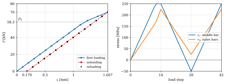
In a finite element model of a real part the same thing happens at every integration point. The yielded zone at a notch is the middle bar, the elastic material around it the outer bars, and the residual stress field after unloading is the plot an FE post-processor shows at the end of a load cycle.
Summary
Elastic deformation is reversible because the material’s structure comes back: bonds return to their spacing, chains coil up again, cell walls unbend. Plastic deformation is the part that does not come back, because dislocations have glided, chains have slid or cells have collapsed. In metals only shear moves dislocations, so their yield criteria ignore the pressure and their plastic flow conserves volume.
The tensile test splits the strain into an elastic part, governed by Hooke’s law, and a plastic part that stays after unloading, 8.17.3. The work done on the material divides into stored elastic energy and dissipated plastic work. Large plastic strains need true stress and true strain, and the hardening curve an FE code asks for is true stress against plastic strain. Three one-dimensional models, perfectly plastic, linearly hardening and nonlinearly hardening, with a fracture strain, cover most engineering use.
In three dimensions the model 8.17.14 consists of the additive split, Hooke’s law on the elastic strain, a yield function, a flow rule normal to the yield surface and a hardening rule that grows the surface with the effective plastic strain. A solver imposes it at every integration point and every step through a return mapping: an elastic trial stress, a check against the yield surface, and a return along the radius when the trial is outside. An explicit solver makes enormous numbers of cheap steps limited by the stable time step, an implicit solver few expensive ones that need the tangent stiffness. A load cycle that causes yielding leaves residual stresses behind, and in the simplest structure they can be computed by hand.
Further reading
Lemaitre and Chaboche cover plasticity, viscoplasticity and damage at the level of a first graduate course, from the mechanisms to the constitutive equations [10]. Ottosen and Ristinmaa derive the yield surfaces, flow rules and hardening models of this chapter in detail and devote a chapter to their numerical integration by return mapping [14]. Simo and Hughes is the standard reference for the algorithms, including the consistent tangent of the radial return and large strains [7]. The LS-DYNA Theory Manual describes the radial return and the material models of the solver used in the course project [12]. Runesson and Larsson’s lecture notes from Chalmers, Constitutive Modeling in Material Mechanics, build plasticity, viscoplasticity and limit loads from one-dimensional models of springs, dampers and sliders such as those of Figure 8.17.1. Gibson and Ashby treat the mechanics of foams [1]. Johan Jansson’s lecture on plasticity for this course at Jönköping University animates the dislocation mechanisms, the yield surfaces and the radial return step by step.
References
[1]
Gibson LJ, Ashby MF. Cellular solids: Structure and properties. 2nd ed. Cambridge: Cambridge University Press; 1997. https://doi.org/10.1017/CBO9781139878326.
[2]
Taylor GI. The mechanism of plastic deformation of crystals. Part I. theoretical. Proceedings of the Royal Society of London Series A 1934;145:362–87. https://doi.org/10.1098/rspa.1934.0106.
[3]
Schmid E, Boas W. Kristallplastizität. Berlin: Springer; 1935. https://doi.org/10.1007/978-3-662-34532-0.
[4]
Hall EO. The deformation and ageing of mild steel: III discussion of results. Proceedings of the Physical Society Section B 1951;64:747–53. https://doi.org/10.1088/0370-1301/64/9/303.
[5]
Petch NJ. The cleavage strength of polycrystals. Journal of the Iron and Steel Institute 1953;174:25–8.
[6]
Hill R. A theory of the yielding and plastic flow of anisotropic metals. Proceedings of the Royal Society of London Series A 1948;193:281–97. https://doi.org/10.1098/rspa.1948.0045.
[7]
Simo JC, Hughes TJR. Computational inelasticity. vol. 7. New York: Springer; 1998. https://doi.org/10.1007/b98904.
[8]
Taylor GI, Quinney H. The latent energy remaining in a metal after cold working. Proceedings of the Royal Society of London Series A 1934;143:307–26. https://doi.org/10.1098/rspa.1934.0004.
[9]
Drucker DC, Prager W. Soil mechanics and plastic analysis or limit design. Quarterly of Applied Mathematics 1952;10:157–65. https://doi.org/10.1090/qam/48291.
[10]
Lemaitre J, Chaboche J-L. Mechanics of solid materials. Cambridge: Cambridge University Press; 1990. https://doi.org/10.1017/CBO9781139167970.
[11]
Wilkins ML. Calculation of elastic-plastic flow. In: Alder B, Fernbach S, Rotenberg M, editors. Methods in computational physics, vol. 3, New York: Academic Press; 1964, p. 211–63.
[12]
Hallquist JO. LS-DYNA theory manual. Livermore, CA: Livermore Software Technology Corporation; 2006.
[13]
Courant R, Friedrichs K, Lewy H. Über die partiellen differenzengleichungen der mathematischen physik. Mathematische Annalen 1928;100:32–74. https://doi.org/10.1007/BF01448839.
[14]
Ottosen NS, Ristinmaa M. The mechanics of constitutive modeling. Amsterdam: Elsevier; 2005.