“The Mathematical Theory of Elasticity is occupied with an attempt to reduce to calculation the state of strain, or relative displacement, within a solid body which is subject to the action of an equilibrating system of forces.”
— A. E. H. Love, A Treatise on the Mathematical Theory of Elasticity, 1892
Solid mechanics, also called mechanics of materials, is the study of the relation between the forces acting on a solid body and the strains and stresses they cause inside it. The practical aim is to dimension parts so that they carry their loads without failing, and to do that we need a measure of how hard a material is being worked.
Force is not that measure. Asking how much force a component can carry before it breaks has no answer, because the answer depends on how much material is there to carry it. A steel cable and a sewing thread both hold ten newtons; only one of them holds ten kilonewtons. Dividing the force by the area over which it acts removes the size of the object and leaves a property of the material, and that quotient is the stress. Chapter 8.3 takes this up properly.
How we shall work
Carrying out analysis by hand as the primary tool for structural design is a thing of the past. The engineer’s job is to study the problem statement and to create and verify the model: to pose the governing equations, to define the load cases through boundary conditions and loads, and to state the assumptions and simplifications that turn a physical object into something computable. The computer’s job is everything after that, the solution of the resulting system of equations, the parameter studies and the visualisations. Machines are better at this than we are, being faster, more accurate and far less prone to sign errors.
What the engineer must bring is computational thinking [see 1], and that is what this part trains. We shall spend our effort on modelling, and we shall spend the time we save on problems that resemble real ones. Traditional courses avoid such problems not because they are unimportant but because they cannot be solved by hand, and what is left after that filtering is a set of academic exercises that no engineer ever meets in practice.
The general case cannot be simplified into a special case that a person can calculate. It is expressed as partial differential equations and solved numerically, in commercial packages such as SolidWorks Simulation, LS-Dyna or Ansys. Those packages implement the finite element method, and applying it to a design problem is called finite element analysis. This part builds the model those packages solve.
Where statics stops
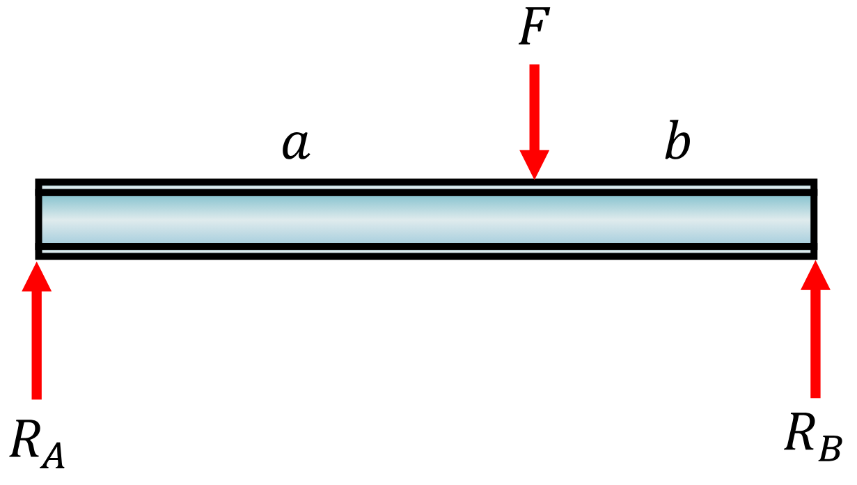
Solid mechanics begins where statics runs out, and it is worth seeing exactly where that is. Consider a rigid beam carrying a force \(F\), resting on two supports separated into the distances \(a\) and \(b\) as in Figure 8.2.1. We want the reaction forces.
Figure 8.2.1: A beam on two supports. Two unknown reactions, two equilibrium equations.
With upward forces and counterclockwise moments positive, force equilibrium in the vertical direction and moment equilibrium about the left support read
\[
\begin{aligned}
R_A + R_B - F &= 0 \\
R_B\,(a + b) - Fa &= 0
\end{aligned}
\]
which are two equations for the two unknown reactions, so the count works out.
R_A, R_B, F, a, b = sp.symbols('R_A R_B F a b', real=True)eqs = [sp.Eq(R_A + R_B - F, 0), # vertical equilibrium sp.Eq(-F*a + R_B*(a + b), 0)] # moments about Asol = sp.solve(eqs, [R_A, R_B], dict=True)[0]sol | la
The reactions are \(R_A = Fb/(a+b)\) and \(R_B = Fa/(a+b)\), and they behave as they should: moving the load towards a support shifts the load onto it, and placing it at the midpoint splits it evenly. This system is statically determinate, meaning that equilibrium alone determines every unknown. Nothing about the material entered the calculation, and nothing needed to: a steel beam and a wooden one of the same geometry carry the same reactions.
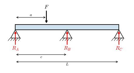
Now add a third support, as in Figure 8.2.2. Physically almost nothing has changed, and mathematically everything has.
Figure 8.2.2: The same beam on three supports. Three unknown reactions, still only two equilibrium equations.
There are now three unknown reactions. Equilibrium still supplies only two equations, because a planar problem with all forces parallel has one force equation and one moment equation and no more. With the middle support at \(c\) and the third at the end \(L\), they read
two equations for three unknowns. Let us ask SymPy for the reactions anyway.
R_C, c, L = sp.symbols('R_C c L', real=True)eqs = [sp.Eq(R_A + R_B + R_C - F, 0), # vertical equilibrium sp.Eq(R_B*c + R_C*L - F*a, 0)] # moments about Asol = sp.solve(eqs, [R_A, R_B, R_C], dict=True)[0]sol | la
\[ \begin{aligned}
R_{A} &= \dfrac{R_{C} \left(L - c\right)}{c} + \dfrac{- F a + F c}{c} \\[9.0pt]
R_{B} &= \dfrac{F a}{c} - \dfrac{L R_{C}}{c}
\end{aligned} \]
SymPy does not fail, and that is the trap. It returns two of the reactions expressed in terms of the third, which is left free. In other words there is not one solution but an infinite family of them, one for every value of \(R_C\) we care to choose. Every member of that family satisfies both equilibrium equations exactly.
We can check that claim by picking two wildly different values and verifying that both are in equilibrium.
numbers = {F: 1000.0, a: 3.0, c: 5.0, L: 10.0}def reactions_for(R_C_value):"""All three reactions once R_C is guessed, and the two equilibrium residuals.""" trial = {R_C: sp.Float(R_C_value)} trial[R_A] = sol[R_A].subs(trial).subs(numbers) trial[R_B] = sol[R_B].subs(trial).subs(numbers) residuals = [sp.simplify(eq.lhs.subs(trial).subs(numbers)) for eq in eqs]return [trial[r] for r in (R_A, R_B, R_C)], residualsrows = []for guess in (0, 400, -250): (R_a, R_b, R_c), residuals = reactions_for(guess) rows.append(rf"R_C = {guess} &\;\Rightarrow\;\;(R_A,\, R_B,\, R_C) = "rf"({float(R_a):.0f},\ {float(R_b):.0f},\ {float(R_c):.0f})~\text{{N}}"rf" &\quad \text{{residuals}} = ({residuals[0]},\,{residuals[1]})")# A cell renders only its last expression, so all three rows go in one call.ltx(r"\\ ".join(rows), aligned=True)
All three sets of reactions balance perfectly, including the two in which one support pulls the beam down rather than holding it up. Statics has no preference between them. The middle support might be carrying nothing at all, or more than the entire applied load, and no amount of equilibrium reasoning will decide which.
A problem of this kind is called statically indeterminate, and the deficit is one equation per redundant support. The count is not a technicality to be worked around; it says that the question we asked has no answer within the model we used.
The missing equation is geometric
The reason statics cannot answer is that we assumed the beam to be rigid, and a rigid beam resting on three supports is an impossible object. If the three supports are perfectly aligned, a rigid beam touches all three and the load distribution is undefined. If one support sits a hair too high, the beam rocks on it and the other two carry nothing. The rigid model is discontinuous here: an arbitrarily small change in geometry produces a completely different answer.
Real beams bend. The middle support pushes up on the beam and the beam pushes back, and how hard it pushes back depends on how far it has been deflected and how stiff it is. That relationship, between a force and a deformation, is the equation statics is missing. Supplying it requires three ingredients that this part develops in turn:
The first is a way to describe deformation, which is the strain of Chapter 8.5 and its tensor generalisation in Chapter 8.7. The second is a way to relate deformation to internal force, which is the material relation measured in Chapter 8.6 and generalised in Chapter 8.8. The third is a way to combine both with equilibrium, which is the pattern named in Chapter 8.9 and applied to a bending member in Chapter 8.14.
With those in hand the beam of Figure 8.2.2 becomes routine. It is a two-segment beam joined at the middle support, exactly the configuration that 8.14.16 handles, and the extra equation comes from requiring the deflection to vanish where the support is. Unlike the rigid answer, the result depends on \(E\) and on the second moment of area, which is the concrete statement that in an indeterminate structure the stiffness decides how the load is shared.
⚠ Note
Statically indeterminate structures are the rule rather than the exception. Welded frames, bolted joints, redundant supports and every closed loop of material produce them. A structure that is determinate has no redundancy, which also means it has no second load path if one member fails.
What is in this part
We begin in one dimension with the normal stress of Chapter 8.3, the shear stress of Chapter 8.4, the strain of Chapter 8.5 and the material data of Chapter 8.6, which together give the vocabulary and the habit of working from a cut and a free body diagram to a stress.
That one-dimensional picture then breaks, deliberately. A cut taken at a different angle through the same bar exposes a different stress, which forces the scalar to become the stress tensor of Chapter 8.7 and the elongation to become the strain tensor. Combined with the generalized Hooke’s law of Chapter 8.8, these close the continuum model of a linearly elastic solid, valid for any geometry and any load.
The remaining chapters are that model specialised. Chapter 8.9 names the three-relation pattern, Chapter 8.10 applies it to an axially loaded member, Chapter 8.11 to a twisted shaft, Chapter 8.12 and Chapter 8.13 to pin-jointed structures, and Chapter 8.14 to a beam in bending. Each is the continuum model plus one assumption about how a cross section moves, and each reduces a system of partial differential equations to something we can solve and differentiate. Where the assumption fails, and it always fails somewhere, finite element analysis takes over.