“Give me a place to stand on, and I can move the earth.”
— Archimedes, as reported by Pappus of Alexandria, c. AD 340
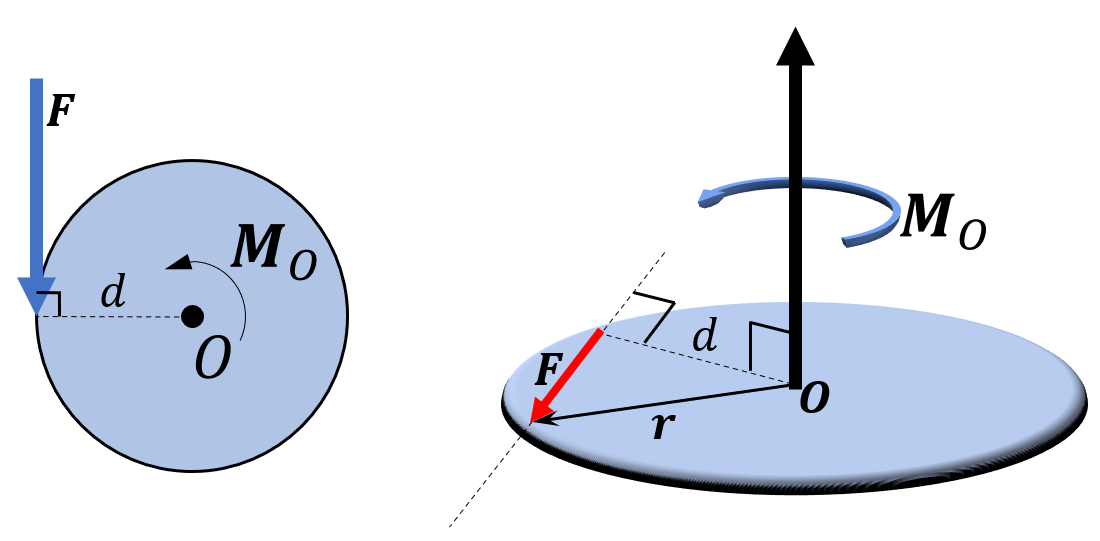
A moment, also known as the torque can be described as a “force to generate a rotation”, as it generates an angular acceleration if not in ballance.
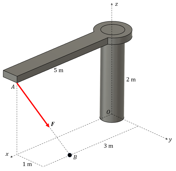
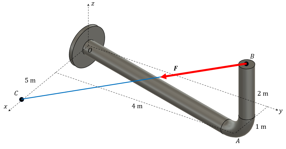
A moment has the unit Newton-meter [ Nm ], it is a vector, and appears around a point as the product of a moment arm (hävarm), \(d\), and an applied force, \(F\), perpendicular to the moment arm, see the figures below.
Moment in 2D and 3D
\[
\boxed{ \boldsymbol M_O = \boldsymbol r \times \boldsymbol F }
\]
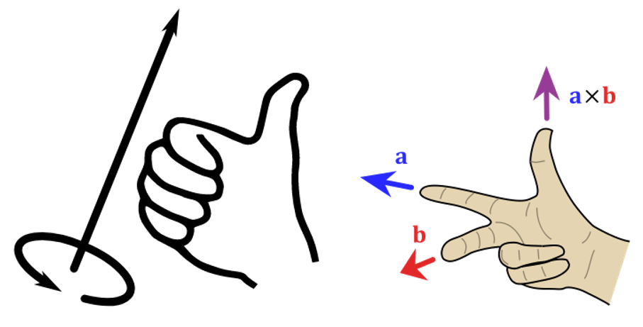
where \(\boldsymbol r\) is known as the moment arm, and \(\boldsymbol F\) is the applied force. The moment arm is the vector from the point of rotation to the line of action of the force. The direction of the moment is determined by the right-hand rule, which states that if you curl your fingers in the direction of rotation, your thumb will point in the direction of the moment.
The scalar counterpart
\[
M = F d
\]
Figure 4.4.1: Two forms of the right-hand rule. Left: when the fingers curl in the sense of rotation, the thumb points along the moment vector. Right: with the index finger along \(\bm a\) and the middle finger along \(\bm b\), the thumb points along \(\bm a \times \bm b\).
We can derive the moment vector from Figure 4.4.2, which lays the components of \(\bm r\) and \(\bm F\) along the axes and builds the three moment components from them.
Figure 4.4.2: The moment of \(\bm F\) about \(O\), component by component. Each moment component turns about its axis, positive by the right-hand rule, and is built from the two force components across that axis and the two arm components that reach them.
The operator \(\times\) is known as the cross product or vector product, and in 3D for a moment arm vector and force vector the physical meaning is a moment vector. The cross product is a vector that is perpendicular to the plane formed by the two vectors being multiplied. The order of operation is important, according to the right-hand rule convention, the moment arm vector is the first vector.
\[
\boldsymbol M = \boldsymbol r \times \boldsymbol F = - \boldsymbol F \times \boldsymbol r
\]
$$ \boldsymbol M = \left[\begin{matrix}0\\0\\30\end{matrix}\right] $$
Note that the \(y\) component in rr can take any value, and the moment around \(z\) will be the same, this is obvious since the \(x\) distance does not change.
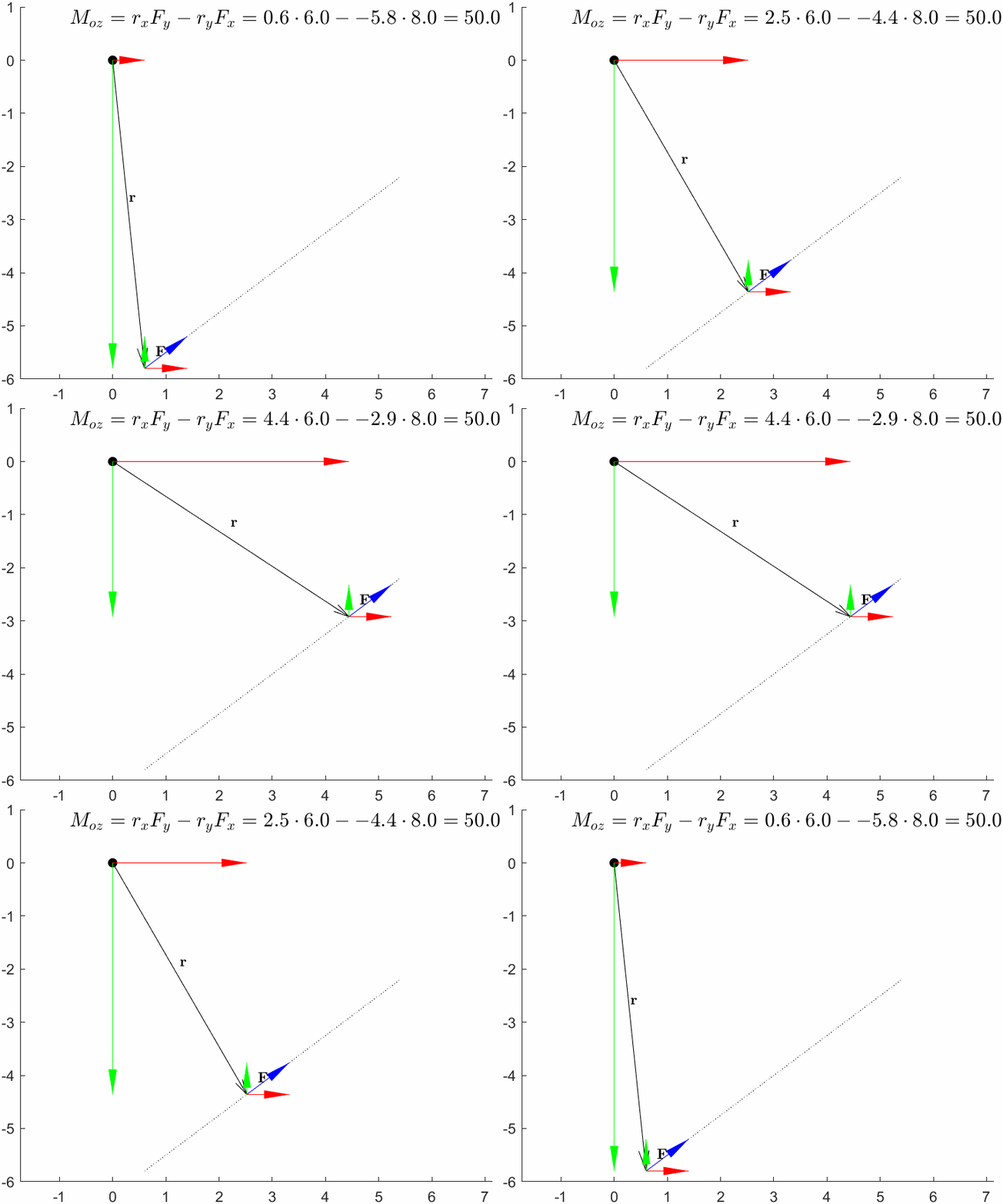
$$ \boldsymbol M = \left[\begin{matrix}0\\0\\50.0\end{matrix}\right] $$
Here we can vary the parameter \(t\) to set the point of application to any point along the line of application and the moment around the \(z\) axis will be unaffected. In fact the can set the parameter \(t\) to a symbolic value and we can see that \(t\) vanishes in the cross product.
t = sp.symbols('t', real=True)rr = rr_OA + t*ee_Frr
\(\displaystyle \left[\begin{matrix}0.8 t + 3\\0.6 t - 4\\0\end{matrix}\right]\)
MM = rr.cross(FF)
$$ \boldsymbol M = \left[\begin{matrix}0\\0\\8.88178419700125 \cdot 10^{-16} t + 50.0\end{matrix}\right] $$
⚠ Note
Here sympy generates numerical round off errors, 10^-16 is a very small number and can be neglected.
Another way of avoiding this floating-point arithmetic is to use the Rational class in sympy, which will keep the numbers as fractions. This is useful when you want to avoid round off errors in your calculations.