6.3  Particle Kinematics

What is kinematics?

Kinematics is the study of motion without regard to what causes it. We describe how a body moves, its position, velocity and acceleration, without asking why it moves. The forces and moments responsible for the motion belong to kinetics, which we treat in later chapters. This separation is useful because the geometry of motion obeys its own rules independently of the forces involved: a particle tracing a circular arc has a centripetal acceleration whether it is a planet in orbit or a ball on a string.

We begin with the simplest case: particle kinematics.

A body whose rotation is insignificant compared to the path its center of gravity travels is called a particle. More precisely, if either the rotational acceleration or the physical size of the body is small enough, we can neglect changes in angular momentum and treat the body as a point mass. The equation of motion then reduces to Newton’s second law,

\[ \sum F = m a \]

and the rotational equation of motion \(\sum M = I \alpha\) can be ignored. Later we will generalize to rigid bodies where rotation matters, but for now these two examples illustrate the distinction:

Figure 6.3.1: The flywheel must be treated as a rigid body; it is being accelerated and de-accelerated, thus it generates a rotational moment around its axis, by design, providing an energy reservoir to the system.
Figure 6.3.2: This marble can be treated as a particle since its rotational speed does not significantly influences its path.

Position vector

Position Vector

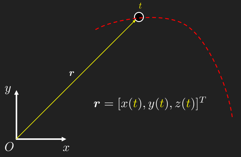
The position of a body’s center of gravity at time \(t\) is described by the position vector \(\boldsymbol{r}(t) = [x(t), y(t), z(t)]^\mathsf{T}\), where each component is a function of the same independent variable \(t\). These components are called coordinate functions, and the curve traced out by \(\boldsymbol{r}(t)\) as \(t\) varies is the path of the particle.

Velocity

Velocity Vector

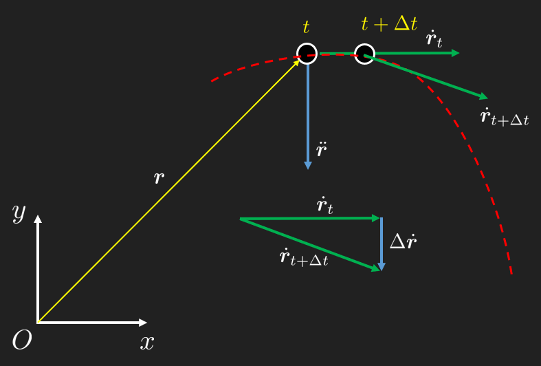
The mean velocity between two positions \(\boldsymbol{r}(t)\) and \(\boldsymbol{r}(t+\Delta t)\) can be described as \(\bar{\boldsymbol{v}} = \frac{\Delta \boldsymbol{r}}{\Delta t}\). In the limit where \(\Delta t \to 0\) we get the time derivate of the position vector, known as the velocity vector

\[ \lim_{\Delta t \to 0} \frac{\Delta \boldsymbol{r}}{\Delta t} = \frac{d\boldsymbol{r}}{dt} =: \dot{\boldsymbol{r}} = \boldsymbol{v} \tag{6.3.1}\]

As can be seen in the animation, the velocity vector \(\dot{\boldsymbol{r}}\) at \(t\) is always tangential to the path.

The dot notation in \(\dot{r}\) or in \(\dot{\ddot{\ddot{\ddot{\ddot{r}}}}} = \frac{d^9}{dt^9}r\) (a.k.a. Newton’s abomination) comes from Newton who studied dynamic problems and needed to develop the mathematics to deal with these problems.
The mathematics came to be known as calculus which was expanded and is really made up by a great many contributors (Leibnitz, Lagrange). see e.g., this video for an historical overview.

The magnitude of the velocity vector, \(|\dot{\boldsymbol{r}}|\), is known as the speed. The difference between velocity and speed being that velocity also contains information about the direction of the object.

Acceleration

Similarly, the acceleration is the time derivative of the velocity,

\[ \lim_{\Delta t \to 0} \frac{\Delta \dot{\boldsymbol{r}}}{\Delta t} = \frac{d\dot{\boldsymbol{r}}}{dt} = \frac{d^2\boldsymbol{r}}{dt^2} =: \ddot{\boldsymbol{r}} = \boldsymbol{a} \tag{6.3.2}\]

Acceleration Vector

Acceleration Animation

From the animation we can see that the acceleration points inward, toward the center of curvature, and that it generally differs in direction from both the position and velocity vectors. The acceleration vector can be decomposed into a tangential and a normal component, \(\boldsymbol{a} = a_t \boldsymbol{e}_t + a_n \boldsymbol{e}_n\). The normal component \(a_n\) is responsible for changes in direction, while the tangential component \(a_t\) is responsible for changes in speed. If the particle speeds up through a curve, so that \(|\dot{\boldsymbol{r}}_1| > |\dot{\boldsymbol{r}}_0|\), a tangential component is present and the resulting acceleration is no longer perpendicular to the velocity. Only when the speed is constant (\(a_t = 0\)) is the acceleration purely normal, that is, perpendicular to the path.
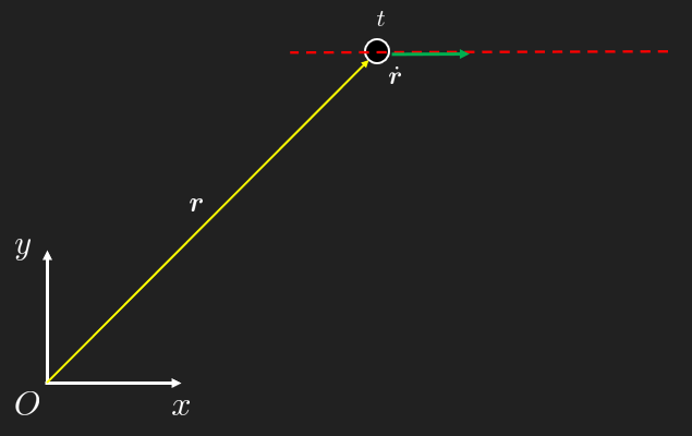
Rectilinear motion

In the special case of rectilinear motion (motion without curvature), such as described in Figure 6.3.3

Figure 6.3.3: Rectilinear Motion

the position vector reduces to a single component, for example \(x(t)\), and the velocity and acceleration reduce to the time derivatives of this single component.

⚠ Note

Using scalar notation \(s = |\boldsymbol{r}|\), \(v = |\dot{\boldsymbol{r}}|\), \(a = |\ddot{\boldsymbol{r}}|\) and eliminating \(dt\) from \(v = ds/dt\) and \(a = dv/dt\) gives

\[ \boxed{a \, ds = v \, dv} \tag{6.3.3}\]

This relation is useful when time is not of interest, but it only applies to rectilinear (or scalar) problems and hides the assumptions behind it. We generally prefer the full vector formulation and the differential equation approach described next.

The proposed working method is described in what follows.

Differential equations

Classical mechanics textbooks often present ready-made formulas for position, velocity and acceleration under specific assumptions (typically constant acceleration). It is usually more tedious to figure out when these formulas are valid than to set up and solve the differential equation directly. We shall therefore work with \(\boldsymbol{r}, \dot{\boldsymbol{r}}\) and \(\ddot{\boldsymbol{r}}\) throughout and treat kinematics problems as ordinary differential equations (ODEs).

Differentiation and integration act componentwise on vectors,

\[ \dot{\boldsymbol{r}}(t) = [\dot x(t), \dot y(t), \dot z(t)]^\mathsf T \quad \text{and} \quad \int \boldsymbol{r}(t) \, dt = \left[\int x(t) \, dt, \int y(t) \, dt, \int z(t) \, dt\right]^\mathsf T \]

so we can formulate our problems in vector form and solve them using either a symbolic ODE solver such as sympy.dsolve() or a numerical integrator such as the Euler method.

Workflow

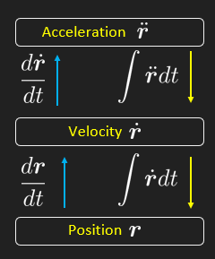
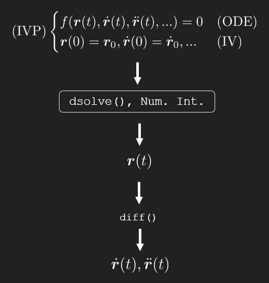
The workflow in computational dynamics is summarized below.

Workflow

To move between position \(\boldsymbol{r}(t)\), velocity \(\dot{\boldsymbol{r}}(t)\) and acceleration \(\ddot{\boldsymbol{r}}(t)\) we differentiate in one direction and integrate in the other. In practice we rarely integrate by hand; instead we solve an ODE whose solution gives \(\boldsymbol{r}(t)\) directly, and then differentiate to obtain the quantities we need. For nonlinear ODEs we typically resort to numerical integration, which generates the velocity \(\dot{\boldsymbol{r}}\) as an intermediate result on the way to the position \(\boldsymbol{r}\).

Newtonian physics is formulated as the second-order differential equation

\[ \sum \boldsymbol{F} = m\ddot{\boldsymbol{r}} \]

but in kinematics we see equally often first-order equations.

IVP

We formulate an ODE that must be (at least piecewise) valid for all \(t\) and apply initial conditions at the start of the analysis, or at some other known state, to fix the unknown constants. The number of constants depends on the order of the differential equation. In this approach, time \(t\) is the central parameter tying \(\boldsymbol{r}\), \(\dot{\boldsymbol{r}}\) and \(\ddot{\boldsymbol{r}}\) together, which is why it often appears in the solution even when we did not explicitly ask for it. This is the nature of Newtonian mechanics: it is inherently transient, meaning the state of the body is known at every instant. As we shall see in later chapters, there are methods that bypass the time dependence when it is not of interest (e.g., 6.3.3), but a complete dynamic analysis always requires solving the ODE.

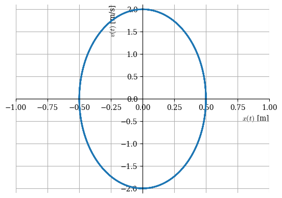
The questions we ask of the model fall into two categories. In the first, the equations are explicitly functions of time, e.g., \(\dot{\boldsymbol{r}}(t)\), so we can evaluate any quantity at a given instant. In the second, we want a quantity expressed as a function of another quantity, for example the velocity at a given position \(\dot{\boldsymbol{r}}(\boldsymbol{r})\), and must solve for the time that is common to both. A useful trick to avoid solving is to simply plot \(\dot{\boldsymbol{r}}(t)\) against \(\boldsymbol{r}(t)\) and read off the answer graphically.

Coordinate systems

Coordinate systems

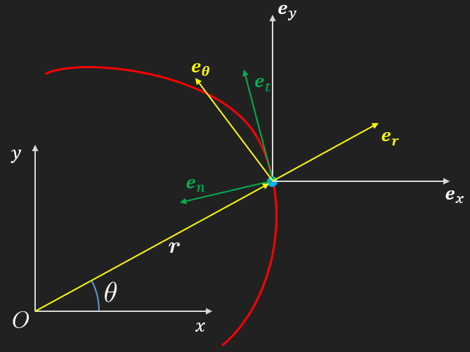
Different coordinate systems align their basis vectors with different aspects of the motion. This alignment often simplifies the resulting expressions, but more importantly, it reveals the physical structure of the problem: polar coordinates naturally separate radial and angular motion, natural coordinates separate speed from curvature, and so on. Whichever system we choose, we should commit to it for the duration of the analysis.

⚠ Note

We can avoid this whole exercise of practicing to compute velocities and acceleration in various bases by just formulating relations in Cartesian coordinates and directly work with the position vector \(\boldsymbol{r}\) which can be easily projected onto any other bases if needed. Let the computer do the tedious mathematics!

We shall here derive the most common coordinate systems and their basis vectors such that this projection can be done. The three systems we consider are:

  • Cartesian, our typical xyz-system with fixed basis vectors \(\boldsymbol{e}_x = [1, 0, 0]^\mathsf{T}\), \(\boldsymbol{e}_y = [0, 1, 0]^\mathsf{T}\) and \(\boldsymbol{e}_z = [0, 0, 1]^\mathsf{T}\).
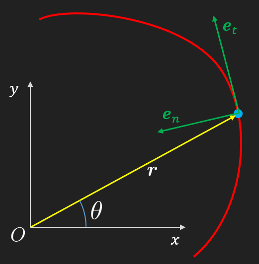
  • Natural (tangent, normal, bi-normal), \(\boldsymbol{e}_t, \boldsymbol{e}_n, \boldsymbol{e}_b\), attached to the particle and aligned with its path.
  • Polar (2D) or cylindrical (3D), \(\boldsymbol{e}_r, \boldsymbol{e}_\theta, \boldsymbol{e}_z\), aligned with the radial direction from a fixed origin.

The Cartesian basis is constant and needs no further discussion. The natural and polar bases, however, rotate as the particle moves, which means their basis vectors are functions of time. This has important consequences when we differentiate position, velocity and acceleration, as we shall see below.

Natural coordinates

The natural coordinate system is attached to the particle and moves with it along its path. This makes it particularly useful when we are interested in how fast the particle travels along the path and how sharply it turns, rather than its absolute position in space.

The first basis vector, the tangent vector \(\boldsymbol{e}_t\), points in the direction the particle is currently moving. Since the velocity \(\dot{\boldsymbol{r}}\) is always tangent to the path, we obtain the tangent direction by normalizing it,

\[ \boxed{\boldsymbol{e}_t = \frac{\dot{\boldsymbol{r}}}{|\dot{\boldsymbol{r}}|} } \]

The second basis vector, the normal vector \(\boldsymbol{e}_n\), points toward the center of curvature, that is, in the direction the path is currently bending. We obtain it from the time derivative of \(\boldsymbol{e}_t\) which, as shown in Section 6.3.8, is always perpendicular to \(\boldsymbol{e}_t\) itself,

\[ \boxed{\boldsymbol{e}_n = \frac{\dot{\boldsymbol{e}}_t}{|\dot{\boldsymbol{e}}_t|}} \]

Together, \(\boldsymbol{e}_t\) and \(\boldsymbol{e}_n\) span the plane in which the path locally curves. The third basis vector, the bi-normal \(\boldsymbol{e}_b\), completes the right-handed system by pointing out of that plane,

\[ \boxed{ \boldsymbol{e}_b := \boldsymbol{e}_t \times \boldsymbol{e}_n } \]

For planar problems (2D) the path always curves in the same plane, so \(\boldsymbol{e}_b = \boldsymbol{e}_z\) throughout the motion.

Polar coordinates

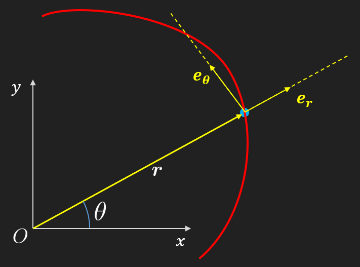
The polar coordinate system is defined relative to a fixed origin. It separates the motion into a radial component (toward or away from the origin) and an angular component (around it), which makes it particularly useful when the radius changes over time or when that change is of interest.

The radial basis vector \(\boldsymbol{e}_r\) points from the origin toward the particle. We obtain it by normalizing the position vector,

\[ \boxed{\boldsymbol{e}_r = \frac{\boldsymbol{r}(t)}{|\boldsymbol{r}(t)|}} \]

The angular basis vector \(\boldsymbol{e}_\theta\) points in the direction of increasing \(\theta\), perpendicular to \(\boldsymbol{e}_r\). As the particle moves, \(\boldsymbol{e}_r\) rotates, and its time derivative (see Section 6.3.8) gives precisely this perpendicular direction,

\[ \boxed{\boldsymbol{e}_\theta = \frac{\dot{\boldsymbol{e}}_r}{|\dot{\boldsymbol{e}}_r|}} \]

In three dimensions a third basis vector \(\boldsymbol{e}_z\) is added along the axis of rotation, giving the cylindrical coordinate system.

The time derivative of a unit vector

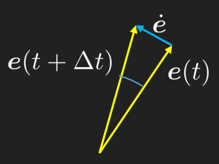
In both the natural and polar coordinate systems we encountered the time derivative of a unit vector, \(\dot{\boldsymbol{e}}\). We now show that this derivative is always perpendicular to the unit vector itself.

A unit vector satisfies \(\boldsymbol{e} \cdot \boldsymbol{e} = 1\) by definition. Differentiating both sides with respect to time and applying the product rule gives

\[ \frac{d}{dt}(\boldsymbol{e} \cdot \boldsymbol{e}) = \dot{\boldsymbol{e}} \cdot \boldsymbol{e} + \boldsymbol{e} \cdot \dot{\boldsymbol{e}} = 2\,\boldsymbol{e} \cdot \dot{\boldsymbol{e}} = 0 \]

and since \(\boldsymbol{e} \cdot \dot{\boldsymbol{e}} = 0\) we conclude that \(\boldsymbol{e} \perp \dot{\boldsymbol{e}}\). Note that \(|\dot{\boldsymbol{e}}| \neq 1\) in general.

Unit Vector Derivative

The figure confirms this geometrically: as \(\Delta t \to 0\), the change \(\Delta\boldsymbol{e}\) becomes perpendicular to \(\boldsymbol{e}\).

Remark 18.1. We verify the result above using \(\boldsymbol{r}(t) = [\cos{\theta(t)}, \sin{\theta(t)}]\).

⚠ Note

Be careful when defining angles as degrees! Angles will be functions of time in what follow, meaning implicit derivation will yield expressions where angles are directly multiplied with distances or velocities, this only works if the angles are defined as radians!

import sympy as sp
from mechanicskit import la, ltx
t = sp.symbols('t', real=True, positive=True)
theta = sp.Function('theta', real=True)(t)

rr = sp.Matrix([sp.cos(theta), sp.sin(theta)])

ltx("\\bm r =", rr)

\[ \bm r =\left[\begin{matrix}\cos{\left(\theta{\left(t \right)} \right)}\\\sin{\left(\theta{\left(t \right)} \right)}\end{matrix}\right] \]

Normalizing gives \(\boldsymbol{e}_r\),

ee_r = sp.trigsimp(rr.normalized())

ltx("\\bm e_r =", ee_r)

\[ \bm e_r =\left[\begin{matrix}\cos{\left(\theta{\left(t \right)} \right)}\\\sin{\left(\theta{\left(t \right)} \right)}\end{matrix}\right] \]

⚠ Note

We cannot simplify the trigonometric expressions if the angle \(\theta\) is not assumed to be a real valued function.

The time derivative of the unit vector \(\boldsymbol{e}_r\) is

ee_r_dot = ee_r.diff(t)
ltx(r"\dot{\bm e}_r =", ee_r_dot, arraystretch=2.5)

\[ {\def\arraystretch{2.5}\dot{\bm e}_r =\left[\begin{matrix}- \sin{\left(\theta{\left(t \right)} \right)} \dfrac{d}{d t} \theta{\left(t \right)}\\\cos{\left(\theta{\left(t \right)} \right)} \dfrac{d}{d t} \theta{\left(t \right)}\end{matrix}\right]} \]

The result is a scaled vector orthogonal to \(\boldsymbol{e}_r\). Note that \(\dot{\theta}\) appears from implicit differentiation, which is why \(|\dot{\boldsymbol{e}}_r| \neq 1\) in general. The factor \(\dot{\theta}\) is the angular velocity \(\omega\), and its sign gives the direction of rotation.

We can therefore write

\[ \boxed{\dot{\boldsymbol{e}}_r = \dot{\theta}\boldsymbol{e}_\theta} \]

and obtain \(\boldsymbol{e}_\theta\) by normalizing \(\dot{\boldsymbol{e}}_r\),

\[ \boxed{\boldsymbol{e}_\theta = \frac{\dot{\boldsymbol{e}}_r}{|\dot{\boldsymbol{e}}_r|}} \]

theta_dot = sp.symbols(r'\dot{\theta}', real=True)
ee_theta = ee_r_dot.normalized().subs(sp.diff(theta, t), theta_dot)
ee_theta = sp.trigsimp(ee_theta)

ltx(r"{\bm e}_\theta =", ee_theta, arraystretch=2.5)

\[ {\def\arraystretch{2.5}{\bm e}_\theta =\left[\begin{matrix}- \dfrac{\dot{\theta} \sin{\left(\theta{\left(t \right)} \right)}}{\left|{\dot{\theta}}\right|}\\\dfrac{\dot{\theta} \cos{\left(\theta{\left(t \right)} \right)}}{\left|{\dot{\theta}}\right|}\end{matrix}\right]} \]

The factor \(\frac{\dot{\theta}}{|\dot{\theta}|}\) is simply the sign of \(\dot{\theta}\), so for \(\dot{\theta} > 0\) we get \(\boldsymbol{e}_\theta = [-\sin\theta, \cos\theta]^\mathsf{T}\). We confirm orthogonality by computing the dot product,

\[ \boldsymbol{e}_r \cdot \boldsymbol{e}_\theta = [\cos\theta, \sin\theta] \cdot [-\sin\theta, \cos\theta] = -\cos\theta\sin\theta + \sin\theta\cos\theta = 0 \]

which verifies that \(\boldsymbol{e}_r \perp \dot{\boldsymbol{e}}_r\) and \(\boldsymbol{e}_r \perp \boldsymbol{e}_\theta\).

Polar coordinates (\(r-\theta\))

We now derive the kinematic equations in polar coordinates. In practice we can formulate \(\dot{\boldsymbol r}\) and \(\ddot{\boldsymbol r}\) in Cartesian coordinates and project onto any basis, so there is no need to memorize the expressions below. The purpose here is to explore the connections between these quantities and their physical meaning.

Polar coordinates

We begin by recalling the basis vectors established earlier,

\[ \boldsymbol{e}_r = \frac{\boldsymbol{r}}{|\boldsymbol{r}|}, \qquad \boldsymbol{e}_\theta = \frac{\dot{\boldsymbol{e}}_r}{|\dot{\boldsymbol{e}}_r|} \]

and writing the position vector as

\[ \boldsymbol{r} = r\boldsymbol{e}_r \]

where \(r = |\boldsymbol{r}|\) is the radial distance from the origin.

Velocity in polar coordinates

Taking the derivative of the position vector using the product rule gives

\[ \dot{\boldsymbol{r}} = \frac{d}{dt}(r(t)\boldsymbol{e}_r(t)) = \dot{r}\boldsymbol{e}_r + r\dot{\boldsymbol{e}}_r \tag{6.3.4}\]

and with \(\dot{\boldsymbol{e}}_r = \dot{\theta}\boldsymbol{e}_\theta\) from the previous section we have

\[ \boxed{\dot{\boldsymbol{r}} = \dot{r}\boldsymbol{e}_r + r\dot{\theta}\boldsymbol{e}_\theta} \]

The quantity \(\omega = \dot{\theta}\) is the angular velocity, and \(v_\theta = r\dot{\theta}\) is the tangential speed. The first term \(\dot{r}\boldsymbol{e}_r\) captures how fast the particle moves toward or away from the origin, while the second term \(r\dot{\theta}\boldsymbol{e}_\theta\) captures how fast it sweeps around it.

Acceleration in polar coordinates

Taking the time derivative of 6.3.4 and applying the product rule to each term gives

\[ \ddot{\boldsymbol{r}} = (\ddot{r}\boldsymbol{e}_r + \dot{r}\dot{\boldsymbol{e}}_r) + (\dot{r}\dot{\theta}\boldsymbol{e}_\theta + r\ddot{\theta}\boldsymbol{e}_\theta + r\dot{\theta}\dot{\boldsymbol{e}}_\theta) \]

We already know that \(\dot{\boldsymbol{e}}_r = \dot{\theta}\boldsymbol{e}_\theta\). By the same argument (differentiating \(\boldsymbol{e}_\theta \cdot \boldsymbol{e}_\theta = 1\)), the time derivative \(\dot{\boldsymbol{e}}_\theta\) must be perpendicular to \(\boldsymbol{e}_\theta\), and direct computation shows \(\dot{\boldsymbol{e}}_\theta = -\dot{\theta}\boldsymbol{e}_r\). Substituting both and collecting terms,

\[ \boxed{\ddot{\boldsymbol{r}} = (\ddot{r} - r\dot{\theta}^2)\boldsymbol{e}_r + (r\ddot{\theta} + 2\dot{r}\dot{\theta})\boldsymbol{e}_\theta} \]

The radial component has two contributions: \(\ddot{r}\) is the acceleration of the particle outward from the origin, while \(r\dot{\theta}^2\) points inward and is the centripetal acceleration that arises from the circular part of the motion. In the angular direction, \(r\ddot{\theta} = r\alpha\) is the angular acceleration and \(2\dot{r}\dot{\theta}\) is the Coriolis term. To see where it comes from, consider a particle moving outward (\(\dot{r} > 0\)) while rotating (\(\dot{\theta} > 0\)). As it moves to a larger radius, it must also increase its tangential speed \(r\dot{\theta}\) just to keep up with the same angular velocity. This “extra” angular acceleration is not due to a change in \(\dot{\theta}\) but due to the radius changing, and it appears twice (factor of 2) because \(\dot{r}\) affects both the transport of existing angular momentum outward and the change of the basis vector \(\boldsymbol{e}_\theta\) itself.

Natural coordinates (\(t-n\))

We now derive the kinematic equations in natural coordinates. The acceleration is particularly revealing in this basis since it splits cleanly into a component along the path (change of speed) and a component perpendicular to it (change of direction). As before, we can always obtain these by projecting the total acceleration onto any basis, so the expressions below need not be memorized.

Natural coordinates

We recall the basis vectors established earlier,

\[ \boldsymbol{e}_t = \frac{\dot{\boldsymbol{r}}}{|\dot{\boldsymbol{r}}|}, \qquad \boldsymbol{e}_n = \frac{\dot{\boldsymbol{e}}_t}{|\dot{\boldsymbol{e}}_t|} \]

Radius of curvature

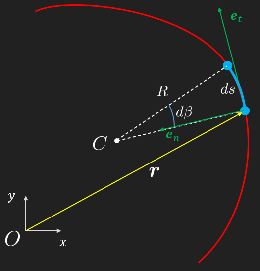
At any point along the path we can fit a circle that locally matches the curvature. The center of this circle is the center of curvature \(C\), and its radius is the radius of curvature \(R\). For an infinitesimal arc angle \(d\beta\), the arc length \(ds\) and the radius are related by

Radius of curvature

The circle arc length relation \(ds = R\,d\beta\), together with the Pythagorean theorem and trigonometry, forms the foundation of our kinematic modelling.

Velocity in natural coordinates

The speed along the path is \(v = |\dot{\boldsymbol{r}}| = \frac{ds}{dt}\), and using the arc length relation \(ds = R\,d\beta\) we get

\[ \dot{\boldsymbol{r}} = v\,\boldsymbol{e}_t = \frac{ds}{dt}\boldsymbol{e}_t = R\dot{\beta}\boldsymbol{e}_t \]

\[ \boxed{v = R\dot{\beta}} \]

This relation is useful when the angular rate \(\dot{\beta}\) is sought.

Angular rate

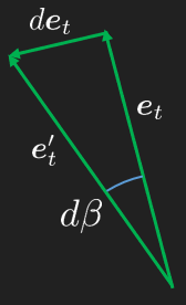
As seen in the figure above, a small change in the angle \(d\beta\) causes a corresponding change \(d\boldsymbol{e}_t\) perpendicular to \(\boldsymbol{e}_t\), that is, in the normal direction \(\boldsymbol{e}_n\). This gives

\[ d\boldsymbol{e}_t = \boldsymbol{e}_n\, d\beta \quad \Rightarrow \quad \dot{\boldsymbol{e}}_t = \dot{\beta}\,\boldsymbol{e}_n = \frac{v}{R}\boldsymbol{e}_n \tag{6.3.5}\]

From 6.3.5 we can also read off the radius of curvature and the angular rate,

\[ R = \frac{v}{|\dot{\boldsymbol{e}}_t|}, \qquad \dot{\beta} = \frac{v}{R} \]

Acceleration in Natural coordinates

Acceleration in Natural Coordinates

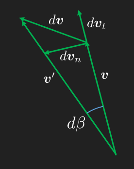
The acceleration vector can be split into a tangential and a normal component, \(\ddot{\boldsymbol{r}} = a_t\boldsymbol{e}_t + a_n\boldsymbol{e}_n\). We find these by differentiating the velocity using the product rule,

\[ \boldsymbol{a} = \ddot{\boldsymbol{r}} = \frac{d}{dt}(v\,\boldsymbol{e}_t) = \dot{v}\,\boldsymbol{e}_t + v\,\dot{\boldsymbol{e}}_t \]

and with 6.3.5 we get

\[ \boxed{\ddot{\boldsymbol{r}} = \underbrace{\dot{v}\,\boldsymbol{e}_t}_{a_t} + \underbrace{\frac{v^2}{R}\boldsymbol{e}_n}_{a_n}} \]

The tangential component \(a_t = \dot{v}\) reflects changes in speed, while the normal component \(a_n = v^2/R\) is the centripetal acceleration directed toward the center of curvature. We always have a normal acceleration as long as the speed is nonzero and the path is curved (\(R < \infty\)). This decomposition will be revisited in the kinetics chapter.

A tiny view on differential geometry

The theory of curves is an extensive topic within the field of differential geometry. Here, we will only introduce some basic concepts, such as the arc length. For a general curve, the arc length may not have a closed-form solution and is found by integrating the speed \(|\dot{\boldsymbol{r}}(t)|\):

\[ s(t) = \int_0^t |\dot{\boldsymbol{r}}(t)| dt \]

Using the arc length \(s\) as the parameter instead of time \(t\) can sometimes lead to simpler expressions for derivatives. However, since \(s\) is itself a function of \(t\), this change of variable does not necessarily simplify computer-based calculations.

Another important concept is curvature, \(\kappa(t) = \frac{1}{R(t)}\). As expected, the curvature approaches zero as the radius of curvature \(R(t)\) tends to infinity, which corresponds to a straight path. The center of curvature, \(\boldsymbol{r}_C(t)\), is given by:

\[ \boldsymbol{r}_C(t) = \boldsymbol{r}(t) + R(t)\boldsymbol{e}_n(t) \]

This point is the center of the osculating circle (a term coined by Leibniz as Circulus Osculans), which is the circle that best approximates the curve at a given point. Natural coordinates are particularly useful for this type of analysis.

⚠ Note

In the special case when \(R(t)\) is constant the bases of polar coordinates coincide with the bases of the natural coordinates.

The torsion of a curve, \(\tau(t)\), measures how sharply it twists out of its plane of curvature. A simple analogy is the pitch of a screw. The derivations for both curvature and torsion can be complex, see e.g., the Frenet-Serret formulas, so the formulas are stated here without proof:

\[ \kappa(t) = \frac{|\dot{\boldsymbol{r}}(t) \times \ddot{\boldsymbol{r}}(t)|}{|\dot{\boldsymbol{r}}(t)|^3} \]

\[ \tau(t) = - \frac{(\dot{\boldsymbol{r}}(t) \times \ddot{\boldsymbol{r}}(t)) \cdot \dot{\ddot{\boldsymbol{r}}}(t)}{|\dot{\boldsymbol{r}}(t) \times \ddot{\boldsymbol{r}}(t)|^2} \]

where \(\dot{\ddot{\boldsymbol{r}}}\) denotes the third-order time derivative of the position vector, also known as jerk or jolt. For the names of higher-order derivatives, see this list.

Remark 18.2. We compute the curvature and torsion for a simple circular path.

Let \(\boldsymbol{r}(t) = R [\cos(t), \sin(t), 0]^\mathsf{T}\), a circle of radius \(R\) in the \(xy\)-plane.

import sympy as sp
from mechanicskit import la, ltx

t = sp.symbols('t', real=True, positive=True)
R = sp.symbols('R', real=True, positive=True)

r = R * sp.Matrix([sp.cos(t), sp.sin(t), 0])

ltx("\\bm r =", r)

\[ \bm r =\left[\begin{matrix}R \cos{\left(t \right)}\\R \sin{\left(t \right)}\\0\end{matrix}\right] \]

r_dot = r.diff(t)
r_ddot = r.diff(t, 2)
r_dddot = r.diff(t, 3)

# kappa = |r_dot x r_ddot| / |r_dot|^3
kappa = sp.simplify((r_dot.cross(r_ddot)).norm() / r_dot.norm()**3)

ltx("\\kappa =", kappa)

\[ \kappa =\dfrac{1}{R} \]

# tau = - (r_dot x r_ddot) . r_dddot / |r_dot x r_ddot|^2
# The cross product r_dot.cross(r_ddot) is not zero, so we can proceed.
tau = sp.simplify(- (r_dot.cross(r_ddot)).dot(r_dddot) / (r_dot.cross(r_ddot)).norm()**2)

ltx("\\tau =", tau)

\[ \tau =0 \]

The curvature is \(\kappa = 1/R\) as expected for a circle, and the torsion is zero since the path lies entirely in the \(xy\)-plane.

Osculating circle

We illustrate the osculating circle on the path \(\boldsymbol{r}(t) = [t,\, \sqrt{t}\sin(2t)]^\mathsf{T}\). The key ingredients are the curvature \(\kappa\), the radius of curvature \(R = 1/\kappa\), the unit normal \(\boldsymbol{e}_n\), and the center of curvature \(\boldsymbol{r}_C = \boldsymbol{r} + R\,\boldsymbol{e}_n\).

Osculating Circle Animation
Code
import numpy as np
import matplotlib.pyplot as plt
from matplotlib.animation import FuncAnimation, PillowWriter

t = sp.symbols('t', real=True, positive=True)
rr = sp.Matrix([t, sp.sqrt(t) * sp.sin(2*t)])

rr_dot = rr.diff(t)
rr_ddot = rr.diff(t, 2)

kappa = (rr_dot[0]*rr_ddot[1] - rr_dot[1]*rr_ddot[0]) / rr_dot.norm()**3
R_curv = 1 / kappa

ee_t = rr_dot / rr_dot.norm()
ee_n = sp.Matrix([-ee_t[1], ee_t[0]])

rr_C = rr + R_curv * ee_n


r_func = sp.lambdify(t, rr, 'numpy')
r_C_func = sp.lambdify(t, rr_C, 'numpy')
R_func = sp.lambdify(t, R_curv, 'numpy')
e_t_func = sp.lambdify(t, ee_t, 'numpy')

fig, ax = plt.subplots(figsize=(8, 6))
fig.patch.set_facecolor('#212121')
ax.set_facecolor('#212121')
ax.set_aspect('equal')
ax.tick_params(axis='x', colors='white')
ax.tick_params(axis='y', colors='white')
for spine in ax.spines.values():
    spine.set_edgecolor('white')

t_vals = np.linspace(0.01, 10, 400)
path = r_func(t_vals)
ax.plot(path[0].flatten(), path[1].flatten(), 'c-')

particle, = ax.plot([], [], 'ro')
circle_line, = ax.plot([], [], 'g-')
tangent_arrow = ax.quiver(0, 0, 0, 0, color='b', scale=1, angles='xy', scale_units='xy')
radius_arrow = ax.quiver(0, 0, 0, 0, color='r', scale=1, angles='xy', scale_units='xy')
ax.set_xlim(0, 10)
ax.set_ylim(-3, 3)
ax.grid(False)

def update(frame):
    pos = r_func(frame)
    center = r_C_func(frame)
    radius = R_func(frame)
    et = e_t_func(frame)
    particle.set_data(pos[0], pos[1])
    tangent_arrow.set_offsets(pos.flatten())
    tangent_arrow.set_UVC(et[0], et[1])
    rv = center - pos
    rv = rv / np.linalg.norm(rv)
    radius_arrow.set_offsets(pos.flatten())
    radius_arrow.set_UVC(rv[0], rv[1])
    theta = np.linspace(0, 2*np.pi, 100)
    circle_line.set_data(center[0] + radius*np.cos(theta), center[1] + radius*np.sin(theta))
    return particle, circle_line, tangent_arrow, radius_arrow

ani = FuncAnimation(fig, update, frames=t_vals, blit=False, interval=50)
ani.save('graphics/kinematics_osculating_circle.gif', writer=PillowWriter(fps=20))
plt.close(fig)

Circular motion

A special case of curvilinear motion is planar circular motion. We study this using polar coordinates and the rotating arm shown below.

Rotating arm

We express the particle’s position as \(\boldsymbol{r} = r(t)[\cos\theta(t), \sin\theta(t)]^\mathsf{T}\).

theta = sp.Function('theta', real=True, positive=True)(t)
r = sp.Function('r', real=True, positive=True)(t)

rr = r * sp.Matrix([sp.cos(theta), sp.sin(theta)])
ltx(r"\bm r =", rr)

\[ \bm r =\left[\begin{matrix}r{\left(t \right)} \cos{\left(\theta{\left(t \right)} \right)}\\r{\left(t \right)} \sin{\left(\theta{\left(t \right)} \right)}\end{matrix}\right] \]

rr_dot = rr.diff(t)
ltx(r"\dot{\bm r} =", rr_dot, arraystretch=2.5)

\[ {\def\arraystretch{2.5}\dot{\bm r} =\left[\begin{matrix}- r{\left(t \right)} \sin{\left(\theta{\left(t \right)} \right)} \dfrac{d}{d t} \theta{\left(t \right)} + \cos{\left(\theta{\left(t \right)} \right)} \dfrac{d}{d t} r{\left(t \right)}\\r{\left(t \right)} \cos{\left(\theta{\left(t \right)} \right)} \dfrac{d}{d t} \theta{\left(t \right)} + \sin{\left(\theta{\left(t \right)} \right)} \dfrac{d}{d t} r{\left(t \right)}\end{matrix}\right]} \]

We clean up by substituting Newton notation for the derivatives.

dot_subs = {
    sp.diff(theta, t, 2): sp.symbols(r'\ddot{\theta}'),
    sp.diff(theta, t):    sp.symbols(r'\dot{\theta}'),
    sp.diff(r, t, 2):     sp.symbols(r'\ddot{r}'),
    sp.diff(r, t):        sp.symbols(r'\dot{r}'),
}

rr_dot = rr_dot.subs(dot_subs)
ltx(r"\dot{\bm r} =", rr_dot, arraystretch=1.5)

\[ {\def\arraystretch{1.5}\dot{\bm r} =\left[\begin{matrix}- \dot{\theta} r{\left(t \right)} \sin{\left(\theta{\left(t \right)} \right)} + \dot{r} \cos{\left(\theta{\left(t \right)} \right)}\\\dot{\theta} r{\left(t \right)} \cos{\left(\theta{\left(t \right)} \right)} + \dot{r} \sin{\left(\theta{\left(t \right)} \right)}\end{matrix}\right]} \]

The acceleration is

rr_ddot = rr.diff(t, 2).subs(dot_subs)
ltx(r"\ddot{\bm r} =", rr_ddot, arraystretch=1.5)

\[ {\def\arraystretch{1.5}\ddot{\bm r} =\left[\begin{matrix}- \ddot{\theta} r{\left(t \right)} \sin{\left(\theta{\left(t \right)} \right)} + \ddot{r} \cos{\left(\theta{\left(t \right)} \right)} - \dot{\theta}^{2} r{\left(t \right)} \cos{\left(\theta{\left(t \right)} \right)} - 2 \dot{\theta} \dot{r} \sin{\left(\theta{\left(t \right)} \right)}\\\ddot{\theta} r{\left(t \right)} \cos{\left(\theta{\left(t \right)} \right)} + \ddot{r} \sin{\left(\theta{\left(t \right)} \right)} - \dot{\theta}^{2} r{\left(t \right)} \sin{\left(\theta{\left(t \right)} \right)} + 2 \dot{\theta} \dot{r} \cos{\left(\theta{\left(t \right)} \right)}\end{matrix}\right]} \]

SymPy handles the tedious differentiation for us. We now define the polar basis vectors and project onto them.

ee_r = sp.Matrix([sp.cos(theta), sp.sin(theta)])
ee_theta = sp.Matrix([-sp.sin(theta), sp.cos(theta)])

where \(\boldsymbol{e}_\theta\) is perpendicular to \(\boldsymbol{e}_r\), rotated 90 degrees counter-clockwise. Projecting onto the polar basis using the dot product (valid since the basis is orthonormal),

rr_dot_polar = sp.simplify(sp.Matrix([ee_r.dot(rr_dot), ee_theta.dot(rr_dot)]))

ltx(r"\dot{\bm r}_{r\theta} =", rr_dot_polar, arraystretch=1.5)

\[ {\def\arraystretch{1.5}\dot{\bm r}_{r\theta} =\left[\begin{matrix}\dot{r}\\\dot{\theta} r{\left(t \right)}\end{matrix}\right]} \]

rr_ddot_polar = sp.simplify(sp.Matrix([ee_r.dot(rr_ddot), ee_theta.dot(rr_ddot)]))

ltx(r"\ddot{\bm r}_{r\theta} =", rr_ddot_polar, arraystretch=1.5)

\[ {\def\arraystretch{1.5}\ddot{\bm r}_{r\theta} =\left[\begin{matrix}\ddot{r} - \dot{\theta}^{2} r{\left(t \right)}\\\ddot{\theta} r{\left(t \right)} + 2 \dot{\theta} \dot{r}\end{matrix}\right]} \]

We recover the same expressions derived by hand in Section 6.3.9.

Special case: Constant radius - circular motion

For constant radius \(r(t) = R\) we set \(\dot{r} = \ddot{r} = 0\) and get the well-known expressions for circular motion.

circ_subs = {sp.symbols(r'\dot{r}'): 0, sp.symbols(r'\ddot{r}'): 0}

ltx(r"\dot{\bm r}_{r\theta} =", rr_dot_polar.subs(circ_subs), arraystretch=1.5)

\[ {\def\arraystretch{1.5}\dot{\bm r}_{r\theta} =\left[\begin{matrix}0\\\dot{\theta} r{\left(t \right)}\end{matrix}\right]} \]

ltx(r"\ddot{\bm r}_{r\theta}  =", rr_ddot_polar.subs(circ_subs), arraystretch=1.5)

\[ {\def\arraystretch{1.5}\ddot{\bm r}_{r\theta} =\left[\begin{matrix}- \dot{\theta}^{2} r{\left(t \right)}\\\ddot{\theta} r{\left(t \right)}\end{matrix}\right]} \]

The first component of the velocity is the radial velocity (zero for circular motion) and the second is the tangential velocity. For the acceleration, the first term is the centripetal acceleration, always pointing toward the center, and the second is the tangential acceleration, which vanishes when the angular velocity is constant.

To summarize planar circular motion: with a constant \(r\), we have \(\dot{r} = \ddot{r} = 0\) and \(\boldsymbol{r} \perp \dot{\boldsymbol{r}}\) since \(\frac{d}{dt}(r^2) = 0 = \frac{d}{dt}(\boldsymbol{r} \cdot \boldsymbol{r}) = \dot{\boldsymbol{r}} \cdot \boldsymbol{r} + \boldsymbol{r} \cdot \dot{\boldsymbol{r}} \Leftrightarrow \boldsymbol{r} \cdot \dot{\boldsymbol{r}} = 0\). Note especially the centripetal acceleration \(-r\dot{\theta}^2\boldsymbol{e}_r\), it is directed in the negative direction of \(\boldsymbol{e}_r\), towards the center of the circle.

If the rotational velocity is constant, i.e., if \(\omega = \dot{\theta} = \text{constant}\) or \(\alpha = \ddot{\theta} = 0\) then we only have centripetal acceleration, caused by a curvilinear motion and perpendicular to the tangent direction, directed inwards, towards the center.

\[ \begin{cases} \boldsymbol{r}(t) = r\,\boldsymbol{e}_r \\ \boldsymbol{v}(t) = r\dot{\theta}\boldsymbol{e}_\theta \\ \boldsymbol{a}(t) = -r\dot{\theta}^2\boldsymbol{e}_r + r\ddot{\theta}\boldsymbol{e}_\theta \end{cases} \]

especially when \(\omega = \dot{\theta} = \text{constant}\)

\[ \begin{cases} \boldsymbol{r}(t) = r\,\boldsymbol{e}_r \\ \boldsymbol{v}(t) = r\omega\boldsymbol{e}_\theta \\ \boldsymbol{a}(t) = -r\omega^2\boldsymbol{e}_r = \{v = |\boldsymbol{v}| = r\omega\} = -\frac{v^2}{r}\boldsymbol{e}_r \end{cases} \]

Circular motion

Note that we can also express \(\boldsymbol{e}_\theta\) using the cross product, \(\boldsymbol{e}_\theta = \boldsymbol{e}_z \times \boldsymbol{e}_r\), which is convenient since circular motion is common and we often have angular velocity as input data. This gives

\[ \boldsymbol{v}(t) = \dot{\theta}\,\boldsymbol{e}_z \times \boldsymbol{r} = r\dot{\theta}\,\boldsymbol{e}_\theta = r\omega\,\boldsymbol{e}_\theta \]

The advantage over explicitly rotating \(\boldsymbol{e}_r\) by 90 degrees is that the cross product automatically gives the correct direction of rotation from the sign of \(\omega\).

Relative motion

Relative motion

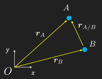
It is often easier to express position, velocity and acceleration relative to some other point rather than the origin. This simplifies the modeling and reflects how engineers typically work: relative measurements are often more practical and more accurate than absolute ones. This approach, called relative motion analysis, will be used extensively in rigid body dynamics.

If we know the position of particle \(B\) and the position of particle \(A\) relative to \(B\), written \(\boldsymbol{r}_{A/B}\) (read: “\(A\) seen from \(B\)”), the absolute position of \(A\) is

\[ \boldsymbol{r}_A = \boldsymbol{r}_B + \boldsymbol{r}_{A/B} \]

It may be more convenient to express \(\boldsymbol{r}_{A/B}\) and \(\boldsymbol{r}_B\) separately than to formulate \(\boldsymbol{r}_A\) directly. Differentiating with respect to time gives

\[ \dot{\boldsymbol{r}}_A = \dot{\boldsymbol{r}}_B + \dot{\boldsymbol{r}}_{A/B} \quad \text{or} \quad \boldsymbol{v}_A = \boldsymbol{v}_B + \boldsymbol{v}_{A/B} \]

and

\[ \ddot{\boldsymbol{r}}_A = \ddot{\boldsymbol{r}}_B + \ddot{\boldsymbol{r}}_{A/B} \quad \text{or} \quad \boldsymbol{a}_A = \boldsymbol{a}_B + \boldsymbol{a}_{A/B} \]

Example 1: Rectilinear motion

The position of a particle moving along a straight line is given by \(s = 2t^3 - 24t + 6\), where \(s\) is in meters and \(t\) in seconds. Determine

  1. the time for the particle to reach a velocity of 72 m/s from its initial condition at \(t = 0\),

  2. the acceleration when \(v = 30\) m/s, and

  3. the net displacement from \(t = 1\) to \(t = 4\).

import sympy as sp
from mechanicskit import la, ltx
t = sp.symbols('t', real=True, positive=True)
s = 2*t**3 - 24*t + 6
v = sp.diff(s, t)
a = sp.diff(v, t)

ltx(r"s(t) =", s, r"\\v(t) =", v, r"\\ a(t) =", a)

\[ s(t) =2 t^{3} - 24 t + 6\\v(t) =6 t^{2} - 24\\ a(t) =12 t \]

(a) Find \(t\) when \(v = 72\) m/s.

t1 = sp.solve(sp.Eq(v, 72), t)
ltx(r"v(t) = 72 \Rightarrow t =", t1)

\[ v(t) = 72 \Rightarrow t =\begin{bmatrix}4\end{bmatrix} \]

(b) Find the acceleration when \(v = 30\) m/s.

t2 = sp.solve(sp.Eq(v, 30), t)
a30 = a.subs(t, t2[0])
ltx(r"v(t) = 30 \Rightarrow t =", t2[0],
    r"\\ a(t_2) =", a30, r"\text{ m/s}^2")

\[ v(t) = 30 \Rightarrow t =3\\ a(t_2) =36\text{ m/s}^2 \]

(c) Net displacement from \(t = 1\) to \(t = 4\).

s4 = s.subs(t, 4)
s1 = s.subs(t, 1)
ds = s4 - s1

ltx(r"s(4) - s(1) =", s4, r"-", s1, r"=", ds, r"\text{ m}")

\[ s(4) - s(1) =38--16=54\text{ m} \]

Example 2: Relative motion

Airplanes in relative motion

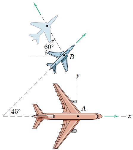
Passengers in an A380 flying east at 800 km/h observe a JAS 39 Gripen passing underneath with a true heading of \(45^\circ\) (north-east). To the passengers, the Gripen appears to move away at \(60^\circ\) as shown. Determine the true speed of the Gripen.

Solution

We have two unknowns: the absolute speed of the Gripen, \(v_B\), and the relative speed observed from the A380, \(v_{B/A}\). The relative motion equation is

\[ \boldsymbol{v}_B = \boldsymbol{v}_A + \boldsymbol{v}_{B/A} \]

Using the known directions,

\[ v_{B}\begin{bmatrix}\cos 45^\circ\\ \sin 45^\circ\end{bmatrix} = \begin{bmatrix}800\\ 0\end{bmatrix} + v_{B/A}\begin{bmatrix}-\cos 60^\circ\\ \sin 60^\circ\end{bmatrix} \]

import sympy as sp
from mechanicskit import la, ltx
v_B, v_BA = sp.symbols('v_B v_{B/A}', real=True, positive=True)
vv_B = v_B * sp.Matrix([sp.cos(sp.rad(45)), sp.sin(sp.rad(45))])
vv_A = sp.Matrix([800, 0])
vv_BA = v_BA * sp.Matrix([-sp.cos(sp.rad(60)), sp.sin(sp.rad(60))])
eq = sp.Eq(vv_B, vv_A + vv_BA)
eq | la(arraystretch=2.5)

\[ {\def\arraystretch{2.5}\left[\begin{matrix}\dfrac{\sqrt{2} v_{B}}{2}\\\dfrac{\sqrt{2} v_{B}}{2}\end{matrix}\right] = \left[\begin{matrix}800 - \dfrac{v_{B/A}}{2}\\\dfrac{\sqrt{3} v_{B/A}}{2}\end{matrix}\right]} \]

sol = sp.solve(eq, (v_B, v_BA))
sol[v_B] | la.evalf(3)

\[ {\def\arraystretch{1.0}717.0} \]

sol[v_BA].evalf(3) | la

\[ {\def\arraystretch{1.0}586.0} \]

The Gripen’s true speed is 717 km/h, and it moves away from the passengers at 586 km/h.

Collision course and relative motion

A striking consequence of relative motion is observed in aviation: when two aircraft are on a collision course, the other aircraft appears stationary in the pilot’s field of view. The relative velocity vector points directly at the observer, so there is no angular motion, only a growing silhouette.

Example 3: Data fitting
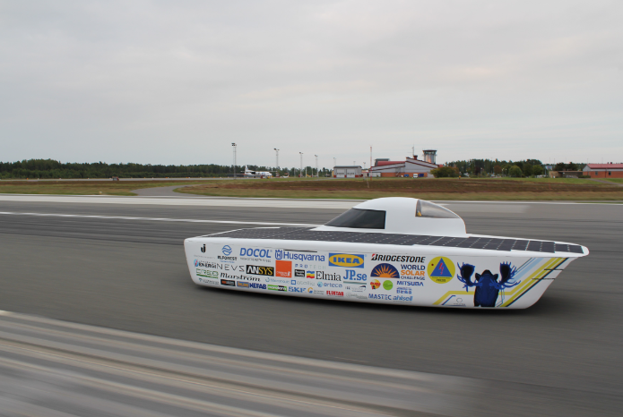
Solar Car

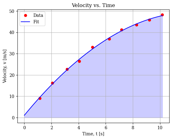
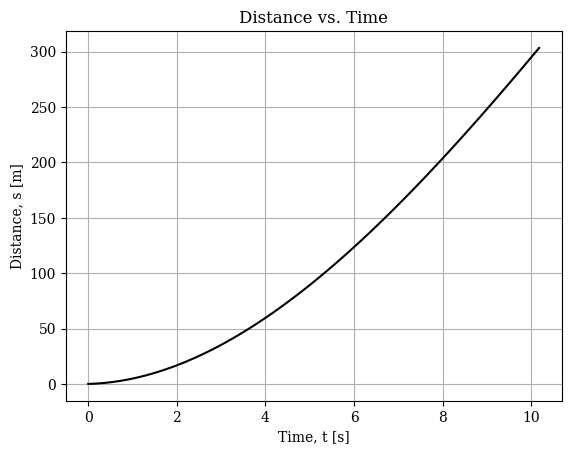
The acceleration performance of a new solar car is being tested at the Jönköping airfield. The JTH students are measuring time against velocity and the data is presented as two vectors. Create a suitable continuous function of the speed and determine how far the car has traveled at the last measurement point. Plot the distance, time and acceleration curves.

Given data:

T=[1.1486, 2.0569, 3.1485, 4.0443, 5.0165, 6.2552, 7.1682, 8.2789, 9.209, 10.175]

V=[9.1023, 16.245, 22.732, 26.446, 33.052, 36.889, 41.304, 43.496, 45.861, 48.319]

Solution

We fit a quadratic polynomial to the data. In ascending powers of \(t\),

\[ v_i = c_0 + c_1 t_i + c_2 t_i^2 \quad \forall\, i \in [1, m] \]

where \(m = 10\) in our case. On matrix form this becomes

\[ \underbrace{\left[\begin{array}{ccc} 1 & t_1 & t_1^2 \\ 1 & t_2 & t_2^2 \\ \vdots & \vdots & \vdots \\ 1 & t_m & t_m^2 \end{array}\right]}_{\bm{X}} \underbrace{\left[\begin{array}{c} c_0 \\ c_1 \\ c_2 \end{array}\right]}_{\bm{c}} = \underbrace{\left[\begin{array}{c} v_1 \\ v_2 \\ \vdots \\ v_m \end{array}\right]}_{\bm{v}} \]

The matrix \(\bm{X}\) is called a Vandermonde matrix. Note that the columns are ordered by ascending powers of \(t\): the first column is \(t^0 = 1\), the second is \(t^1\), the third is \(t^2\). This means \(c_0\) is the constant term, \(c_1\) the linear coefficient, and \(c_2\) the quadratic coefficient, that is, c[i] multiplies \(t^i\).

Since we have more equations (\(m = 10\)) than unknowns (\(n = 3\)), the system is overdetermined and has no exact solution. Instead we seek the \(\bm{c}\) that minimizes the squared error,

\[ E(\bm{c}) = ||\bm{X}\bm{c} - \bm{v}||^2 = (\bm{X}\bm{c} - \bm{v})^\mathsf{T}(\bm{X}\bm{c} - \bm{v}) \]

Expanding and differentiating with respect to \(\bm{c}\) gives

\[ \frac{\partial E}{\partial \bm{c}} = 2\bm{X}^\mathsf{T}\bm{X}\bm{c} - 2\bm{X}^\mathsf{T}\bm{v} = \bm{0} \]

which yields the normal equations,

\[ \boxed{\bm{c} = (\bm{X}^\mathsf{T} \bm{X})^{-1} \bm{X}^\mathsf{T} \bm{v}} \]

import numpy as np
from mechanicskit import la, ltx


# Given data:
T = np.array([1.1486, 2.0569, 3.1485, 4.0443, 5.0165, 6.2552, 7.1682, 8.2789, 9.209, 10.175])
V = np.array([9.1023, 16.245, 22.732, 26.446, 33.052, 36.889, 41.304, 43.496, 45.861, 48.319])

# np.vander builds the Vandermonde matrix
# increasing=True gives columns [1, t, t^2], matching c_0 + c_1*t + c_2*t^2
X = np.vander(T, 3, increasing=True)

ltx(r"\bm X =", X, show_shape=True)

\[ \bm X =\begin{bmatrix}1.00 & 1.15 & 1.32 \\ 1.00 & 2.06 & 4.23 \\ 1.00 & 3.15 & 9.91 \\ 1.00 & 4.04 & 16.36 \\ 1.00 & 5.02 & 25.17 \\ 1.00 & 6.26 & 39.13 \\ \vdots & \vdots & \vdots \\ 1.00 & 10.18 & 103.53\end{bmatrix}_{10 \times 3} \]

The following python code implements \(\mathbf{c}=\left(\mathbf{X}^T \mathbf{X}\right)^{-1} \mathbf{X}^T \mathbf{v}\) literally

c = np.linalg.solve(X.T @ X, X.T @ V)
ltx(r"\bm c =", c, arraystretch=1.0, show_shape=True)

\[ {\def\arraystretch{1.0}\bm c =\begin{bmatrix}1.06 \\ 7.75 \\ -0.31\end{bmatrix}_{3 \times 1}} \]

But doing this manually is tedious and error prone, instead we should use the least squares solver in numpy, numpy.linalg.lstsq

c = np.linalg.lstsq(X, V)[0]

c | la(show_shape=True)

\[ {\def\arraystretch{1.0}\begin{bmatrix} 1.06 \\ 7.75 \\ -0.31 \end{bmatrix}_{3 \times 1}} \]

import sympy as sp
t = sp.Symbol('t')

# Since X has columns [1, t, t^2], c[i] multiplies t^i
v = c[0] + c[1]*t + c[2]*t**2

ltx(r"v(t) =", v, precision=3)

\[ v(t) =- 0.31 t^{2} + 7.75 t + 1.06 \]

We now have a continuous function \(v(t)\) that we can differentiate and integrate symbolically.

Code
import matplotlib.pyplot as plt

v_func = sp.lambdify(t, v, 'numpy')
tn = np.linspace(0, max(T), 100)
vn = v_func(tn)

fig, ax = plt.subplots()
ax.plot(T, V, 'ro', label='Data')
ax.plot(tn, vn, 'b-', label='Fit')
ax.set(xlabel='Time, t [s]', ylabel='Velocity, v [m/s]', title='Velocity vs. Time')
ax.grid(True)
ax.legend()
ax.fill_between(tn, vn, color='b', alpha=0.2)
plt.show()

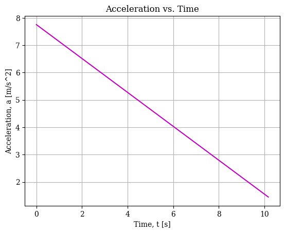
# Acceleration is the derivative of velocity
a = sp.diff(v, t)
ltx(r"a(t) =", a, precision=3)

\[ a(t) =7.75 - 0.62 t \]

Code
# Plot acceleration
an = sp.lambdify(t, a, 'numpy')(tn)
fig, ax = plt.subplots()
ax.plot(tn, an, 'm-')
ax.set(xlabel='Time, t [s]', ylabel='Acceleration, a [m/s^2]', title='Acceleration vs. Time')
ax.grid(True)
plt.show()

# Total distance is the integral of velocity
s_tot = sp.integrate(v, (t, 0, max(T)))

ltx(r"s_{tot} = \int_0^{10.175} v(t)\, dt =", s_tot, precision=4)

\[ s_{tot} = \int_0^{10.175} v(t)\, dt =303.4 \]

s = sp.integrate(v)

ltx(r"s(t) =", s, precision=3)

\[ s(t) =- 0.103 t^{3} + 3.88 t^{2} + 1.06 t \]

Code
sn = sp.lambdify(t, s, 'numpy')(tn)
fig, ax = plt.subplots()
ax.plot(tn, sn, 'k-')
ax.set(xlabel='Time, t [s]', ylabel='Distance, s [m]', title='Distance vs. Time')
ax.grid(True)
plt.show()

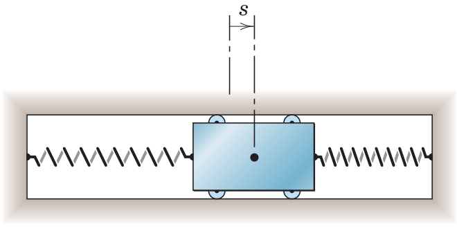
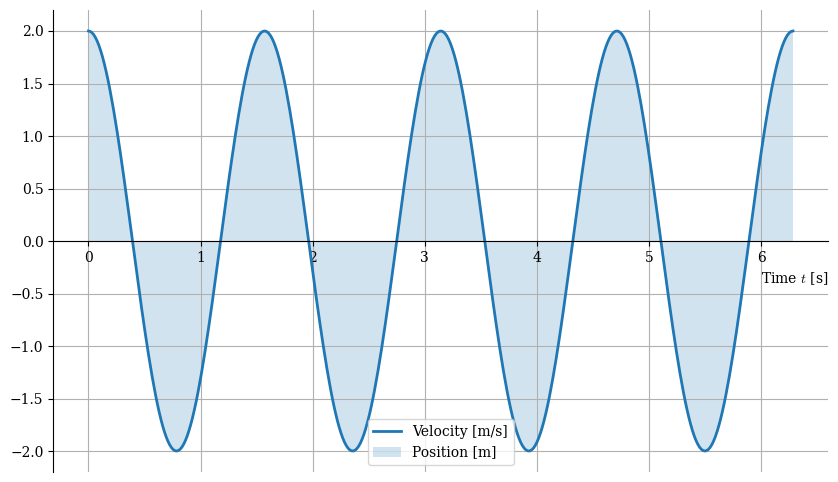
Example 4: Oscillating slider

A spring-mounted slider moves along the \(x\)-axis with initial velocity \(v_0 = 2\) m/s as it crosses the mid-position where \(s = 0\) at \(t = 0\). The two springs exert a retarding force proportional to the displacement, giving an acceleration \(a = -k^2 s\) with \(k = 4\). Determine the displacement, velocity and acceleration of the slider.

Oscillating slider
k, v0 = sp.symbols('k v0', positive=True)
x = sp.Function('x')(t)

DE = sp.Eq(x.diff(t, 2), -k**2 * x)
ICs = {x.subs(t, 0): 0, x.diff(t).subs(t, 0): v0}

DE | la

\[ {\def\arraystretch{1.0}\dfrac{d^{2}}{d t^{2}} x{\left(t \right)} = - k^{2} x{\left(t \right)}} \]

x_sol = sp.simplify(sp.dsolve(DE, ics=ICs).rhs)
ltx(r"x(t) =", x_sol)

\[ x(t) =\dfrac{v_{0} \sin{\left(k t \right)}}{k} \]

v_sol = x_sol.diff(t)
a_sol = v_sol.diff(t)

ltx(r"v(t) =", v_sol)

\[ v(t) =v_{0} \cos{\left(k t \right)} \]

Code

ltx(r"a(t) =", a_sol)

\[ a(t) =- k v_{0} \sin{\left(k t \right)} \]

data = {k: 4, v0: 2}
x_n = x_sol.subs(data)
v_n = v_sol.subs(data)
a_n = a_sol.subs(data)

ltx(r"x(t) =", x_n, r",\quad v(t) =", v_n, r",\quad a(t) =", a_n)

\[ x(t) =\dfrac{\sin{\left(4 t \right)}}{2},\quad v(t) =2 \cos{\left(4 t \right)},\quad a(t) =- 8 \sin{\left(4 t \right)} \]

Code
t1 = 2 * np.pi
t_vals = np.linspace(0, t1, 400)

x_func = sp.lambdify(t, x_n, 'numpy')
v_func = sp.lambdify(t, v_n, 'numpy')
a_func = sp.lambdify(t, a_n, 'numpy')

fig, ax = plt.subplots(figsize=(10, 6))
ax.plot(t_vals, v_func(t_vals), linewidth=2, label='Velocity [m/s]')
ax.fill_between(t_vals, v_func(t_vals), alpha=0.2, label='Position [m]')
ax.spines['bottom'].set_position('zero')
ax.spines['right'].set_color('none')
ax.spines['top'].set_color('none')
ax.set_xlabel(r'Time $t$ [s]', loc='right')
ax.legend()
ax.grid(True)
plt.show()

The total area under the velocity curve is the distance the slider has traveled, which for \(t = 2\pi\) is 2 m. But the signed area is zero, since the slider returns to its starting position after \(2\pi\) seconds, \(x(2\pi) = 0\) m.

signed_area = sp.integrate(v_n, (t, 0, 2*sp.pi))
total_distance = sp.integrate(sp.Abs(v_n), (t, 0, 2*sp.pi))

ltx(r"\int_0^{2\pi} v\, dt =", signed_area,
    r",\qquad \int_0^{2\pi} |v|\, dt =", total_distance)

\[ \int_0^{2\pi} v\, dt =0,\qquad \int_0^{2\pi} |v|\, dt =2 \]

Finally, plotting \(v(t)\) against \(x(t)\) gives the phase portrait: an ellipse, characteristic of simple harmonic motion.

Code
fig, ax = plt.subplots()
ax.plot(x_func(t_vals), v_func(t_vals), linewidth=2)
ax.spines['bottom'].set_position('zero')
ax.spines['left'].set_position('zero')
ax.spines['right'].set_color('none')
ax.spines['top'].set_color('none')
ax.set_xlabel(r'$x(t)$ [m]', loc='right')
ax.set_ylabel(r'$v(t)$ [m/s]', loc='top')
# ax.set_aspect('equal')
ax.set_xlim(-1, 1)
ax.set_ylim(-2.1, 2.1)
ax.grid(True)
plt.show()

Example 5: Piecewise functions

We have noticed the position of a particular nice motorcycle,

\[ x(t) = \begin{cases} t^2 & 0 \le t < 10 \\ 20t - 100 & t \ge 10 \end{cases} \]

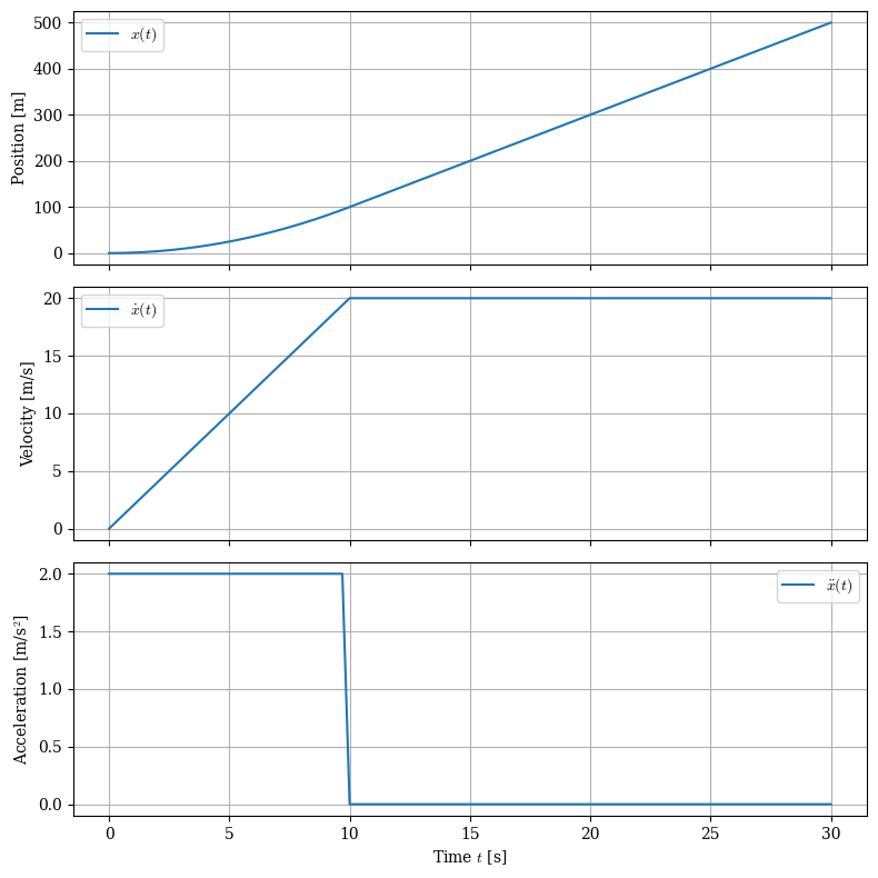
Plot its velocity and acceleration curves for \(t \in [0, 30]\) s.

Solution

We define the piecewise position function and differentiate to obtain velocity and acceleration. Note that at \(t = 10\) the two pieces meet: \(10^2 = 100 = 20 \cdot 10 - 100\), so the position is continuous. The velocity transitions from \(2t = 20\) m/s to a constant 20 m/s, which is also continuous. The acceleration, however, jumps from 2 m/s\(^2\) to 0.

x = sp.Piecewise((t**2, t < 10), (20*t - 100, True))
ltx(r"x(t) =", x)

\[ x(t) =\begin{cases} t^{2} & \text{for}\: t < 10 \\20 t - 100 & \text{otherwise} \end{cases} \]

x_dot = sp.diff(x, t)
x_ddot = sp.diff(x, t, 2)

ltx(r"\dot x(t) =", x_dot, r",\quad\ddot x(t) =", x_ddot)

\[ \dot x(t) =\begin{cases} 2 t & \text{for}\: t < 10 \\20 & \text{otherwise} \end{cases},\quad\ddot x(t) =\begin{cases} 2 & \text{for}\: t < 10 \\0 & \text{otherwise} \end{cases} \]

Code
from mechanicskit import fplot

fig, axes = plt.subplots(3, 1, figsize=(8, 8), sharex=True)

fplot(x, (t, 0, 30), ax=axes[0], label=r'$x(t)$')
axes[0].set_ylabel('Position [m]')
axes[0].legend()
axes[0].grid(True)

fplot(x_dot, (t, 0, 30), ax=axes[1], label=r'$\dot x(t)$')
axes[1].set_ylabel('Velocity [m/s]')
axes[1].legend()
axes[1].grid(True)

fplot(x_ddot, (t, 0, 30), ax=axes[2], label=r'$\ddot x(t)$')
axes[2].set_ylabel(r'Acceleration [m/s$^2$]')
axes[2].set_xlabel('Time $t$ [s]')
axes[2].legend()
axes[2].grid(True)

fig.tight_layout()
plt.show()

Example 6: Solving an ODE using Euler’s method

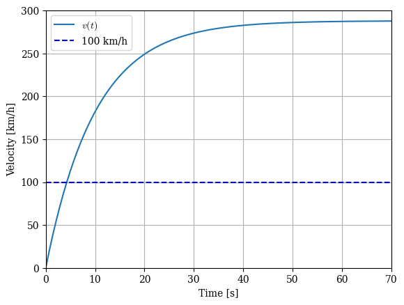
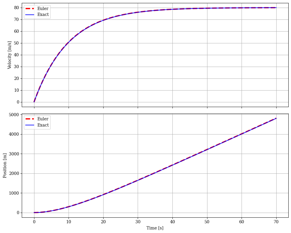
A sports car manufacturer is limiting the power for one of the models by limiting the fuel consumption when the throttle is fully engaged such that the acceleration at any moment is proportional with the constant \(k = 0.1\) s\(^{-1}\) with respect to the difference in wanted top speed \(v_1 = 80\) m/s and the current speed \(v\). Assume the car starts from rest and the driver puts the pedal to the metal.

  • Draw the distance and velocity curves
  • How long does it take to reach top speed and how far has the car traveled?
  • What is the 0-100 km/h time and distance?

Solution

From the problem description we formulate the ODE with initial conditions,

\[ \ddot{x}(t) = k(v_1 - \dot{x}(t)), \quad \dot{x}(0) = 0, \quad x(0) = 0 \]

Symbolic solution

x = sp.Function('x')(t)
v1, k = sp.Rational(80), sp.Rational(1, 10)

DE = sp.Eq(x.diff(t, 2), k * (v1 - x.diff(t)))
ICs = {x.subs(t, 0): 0, x.diff(t).subs(t, 0): 0}

x_sol = sp.dsolve(DE, ics=ICs).rhs
v_sol = x_sol.diff(t)

ltx(r"x(t) =", x_sol, r",\quad v(t) =", v_sol)

\[ x(t) =80 t - 800 + 800 e^{- \dfrac{t}{10}},\quad v(t) =80 - 80 e^{- \dfrac{t}{10}} \]

Code
from mechanicskit import fplot

fig, ax = plt.subplots()
fplot(v_sol * sp.Rational(36, 10), (t, 0, 70), ax=ax, label=r'$v(t)$')
ax.axhline(100, color='b', linestyle='--', label='100 km/h')
ax.set(xlabel='Time [s]', ylabel='Velocity [km/h]')
ax.set_xlim(0, 70)
ax.set_ylim(0, 300)
ax.legend()
ax.grid(True)
plt.show()

How long to reach top speed? Since \(v(t) = 80(1 - e^{-t/10})\) approaches 80 m/s asymptotically, we never truly reach it. In practice we can ask when \(v = 0.99 \cdot v_1\).

t_99 = sp.solve(sp.Eq(v_sol, sp.Rational(99, 100) * v1), t)[0]
x_99 = x_sol.subs(t, t_99)

ltx(r"t_{99\%} =", t_99, r"\text{ s} \approx", t_99.evalf(4), r"\text{ s}")
ltx(r"x(t_{99\%}) =", x_99.evalf(4), r"\text{ m}")

\[ x(t_{99\%}) =2892.0\text{ m} \]

# 100 km/h = 100/3.6 m/s
v_100kmh = sp.Rational(1000, 36)
t_100 = sp.solve(sp.Eq(v_sol, v_100kmh), t)[0]
x_100 = x_sol.subs(t, t_100)

ltx(r"t_{0-100} =", t_100.evalf(4), r"\text{ s}")
ltx(r"x_{0-100} =", x_100.evalf(4), r"\text{ m}")

\[ x_{0-100} =63.44\text{ m} \]

Numerical solution using the Euler forward method

We approximate the derivatives using finite differences,

\[ \ddot{x} \approx \frac{\dot{x}_{i+1} - \dot{x}_i}{\Delta t} = k(v_1 - \dot{x}_i) \quad \Rightarrow \quad \dot{x}_{i+1} = \dot{x}_i + k(v_1 - \dot{x}_i)\Delta t \]

\[ \dot{x} \approx \frac{x_{i+1} - x_i}{\Delta t} \quad \Rightarrow \quad x_{i+1} = x_i + \dot{x}_{i+1} \Delta t \]

dt = 0.1
t_end = 70
n = int(t_end / dt) + 1

t_euler = np.zeros(n)
x_euler = np.zeros(n)
v_euler = np.zeros(n)

k_val, v1_val = 0.1, 80

for i in range(n - 1):
    v_euler[i+1] = v_euler[i] + k_val * (v1_val - v_euler[i]) * dt
    x_euler[i+1] = x_euler[i] + v_euler[i+1] * dt
    t_euler[i+1] = t_euler[i] + dt
Code
x_exact = sp.lambdify(t, x_sol, 'numpy')
v_exact = sp.lambdify(t, v_sol, 'numpy')

fig, (ax1, ax2) = plt.subplots(2, 1, figsize=(10, 8), sharex=True)

ax1.plot(t_euler, v_euler, 'r--', lw=3, label='Euler')
ax1.plot(t_euler, v_exact(t_euler), 'b-', label='Exact')
ax1.set_ylabel('Velocity [m/s]')
ax1.legend()
ax1.grid(True)

ax2.plot(t_euler, x_euler, 'r--', lw=3, label='Euler')
ax2.plot(t_euler, x_exact(t_euler), 'b-', label='Exact')
ax2.set_ylabel('Position [m]')
ax2.set_xlabel('Time [s]')
ax2.legend()
ax2.grid(True)

fig.tight_layout()
plt.show()

Example 7: Curvilinear motion in polar coordinates

A particle \(B\) is confined to the radial groove of a rotating arm. The angular position and radial distance are given by

\[ \theta(t) = 0.2t + 0.02t^3, \qquad r(t) = 0.2 + 0.04t^2 \]

Analyse the motion of the particle in Cartesian and polar coordinates for \(t \in [0, 5]\) s.

Solution

We express the position in Cartesian form, differentiate, then project onto the polar basis to obtain the radial and angular components.

Code
theta = sp.Rational(1, 5)*t + sp.Rational(1, 50)*t**3
r = sp.Rational(1, 5) + sp.Rational(1, 25)*t**2

rr = r * sp.Matrix([sp.cos(theta), sp.sin(theta)])
ltx(r"\theta(t) =", theta, r",\qquad r(t) =", r)

\[ \theta(t) =\dfrac{t^{3}}{50} + \dfrac{t}{5},\qquad r(t) =\dfrac{t^{2}}{25} + \dfrac{1}{5} \]

Code
rr_dot = rr.diff(t)
rr_ddot = rr.diff(t, 2)

We define the polar basis and project the Cartesian velocity and acceleration onto it.

Code
ee_r = sp.Matrix([sp.cos(theta), sp.sin(theta)])
ee_theta = sp.Matrix([-sp.sin(theta), sp.cos(theta)])

v_polar = sp.trigsimp(sp.Matrix([ee_r.dot(rr_dot), ee_theta.dot(rr_dot)]))
a_polar = sp.trigsimp(sp.Matrix([ee_r.dot(rr_ddot), ee_theta.dot(rr_ddot)]))

ltx(r"\dot{\bm r}_{r\theta} =", v_polar, r",\quad \ddot{\bm r}_{r\theta} =", a_polar, arraystretch=2.0)

\[ {\def\arraystretch{2.0}\dot{\bm r}_{r\theta} =\left[\begin{matrix}\dfrac{2 t}{25}\\\dfrac{3 t^{4}}{1250} + \dfrac{t^{2}}{50} + \dfrac{1}{25}\end{matrix}\right],\quad \ddot{\bm r}_{r\theta} =\left[\begin{matrix}- \dfrac{9 t^{6}}{62500} - \dfrac{21 t^{4}}{12500} - \dfrac{4 t^{2}}{625} + \dfrac{9}{125}\\\dfrac{t \left(9 t^{2} + 35\right)}{625}\end{matrix}\right]} \]

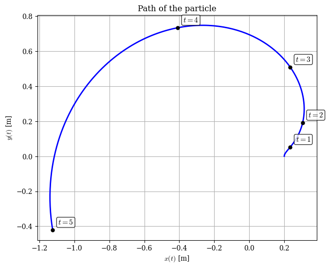
We can verify: \(\dot{r} = 0.08t\) and \(r\dot{\theta} = (0.2 + 0.04t^2)(0.2 + 0.06t^2)\), consistent with the general polar velocity formula \(\dot{\boldsymbol{r}} = \dot{r}\boldsymbol{e}_r + r\dot{\theta}\boldsymbol{e}_\theta\).

Code
rr_func = sp.lambdify(t, rr, 'numpy')
rr_dot_func = sp.lambdify(t, rr_dot, 'numpy')
rr_ddot_func = sp.lambdify(t, rr_ddot, 'numpy')

t_vals = np.linspace(0, 5, 300)
path = np.array([rr_func(ti).flatten() for ti in t_vals])

fig, ax = plt.subplots(figsize=(8, 6))
ax.plot(path[:, 0], path[:, 1], 'b-', linewidth=2)
ax.set_aspect('equal')
ax.set_xlabel(r'$x(t)$ [m]')
ax.set_ylabel(r'$y(t)$ [m]')
ax.set_title('Path of the particle')
ax.grid(True)

# Mark integer time points
for ti in [1, 2, 3,4,5]:
    pos = rr_func(ti).flatten()
    ax.plot(pos[0], pos[1], 'ko', markersize=5)
    ax.annotate(f'$t={ti}$', pos, textcoords='offset points',
               xytext=(8, 8), fontsize=11,
               bbox=dict(boxstyle='round,pad=0.2', fc='white', alpha=0.8))

plt.show()

Code
from matplotlib.animation import FuncAnimation, FFMpegWriter

# Precompute component curves
t_plot = np.linspace(0.1, 5, 300)
vx = np.array([rr_dot_func(ti).flatten()[0] for ti in t_plot])
vy = np.array([rr_dot_func(ti).flatten()[1] for ti in t_plot])
ax_vals = np.array([rr_ddot_func(ti).flatten()[0] for ti in t_plot])
ay = np.array([rr_ddot_func(ti).flatten()[1] for ti in t_plot])

fig = plt.figure(figsize=(14, 6))
ax_path = fig.add_subplot(121)
ax_comp = fig.add_subplot(122)

# Left: path + arrows
ax_path.plot(path[:, 0], path[:, 1], 'b-', linewidth=1, alpha=0.4)
ax_path.set_aspect('equal')
ax_path.set_xlabel(r'$x$ [m]')
ax_path.set_ylabel(r'$y$ [m]')
ax_path.grid(True)
ax_path.set_xlim(-1.5, 0.7)
ax_path.set_ylim(-0.5, 1.3)
ax_path.set_title('Path')

dot, = ax_path.plot([], [], 'ko', markersize=6)
v_arrow = ax_path.annotate('', xy=(0, 0), xytext=(0, 0),
    arrowprops=dict(arrowstyle='->', color='blue', lw=2))
a_arrow = ax_path.annotate('', xy=(0, 0), xytext=(0, 0),
    arrowprops=dict(arrowstyle='->', color='red', lw=2))

# Right: component curves (faint background)
ax_comp.plot(t_plot, vx, 'b-', alpha=0.3, label=r'$\dot x$')
ax_comp.plot(t_plot, vy, 'r-', alpha=0.3, label=r'$\dot y$')
ax_comp.plot(t_plot, ax_vals, 'b--', alpha=0.3, label=r'$\ddot x$')
ax_comp.plot(t_plot, ay, 'r--', alpha=0.3, label=r'$\ddot y$')
ax_comp.set_xlabel(r'$t$ [s]')
ax_comp.set_title('Components')
ax_comp.grid(True)
ax_comp.legend(loc='upper left')

dot_vx, = ax_comp.plot([], [], 'bo', markersize=6)
dot_vy, = ax_comp.plot([], [], 'ro', markersize=6)
dot_ax, = ax_comp.plot([], [], 'b^', markersize=6)
dot_ay, = ax_comp.plot([], [], 'r^', markersize=6)
time_line = ax_comp.axvline(0, color='k', alpha=0.3, linestyle=':')

v_scale = 0.3 / 1.5
a_scale = 0.3 / 2.5
frames = np.linspace(0.1, 5, 200)

def update(ti):
    pos = rr_func(ti).flatten()
    vel = rr_dot_func(ti).flatten()
    acc = rr_ddot_func(ti).flatten()
    vs = vel * v_scale
    acs = acc * a_scale
    dot.set_data([pos[0]], [pos[1]])
    v_arrow.xy = (pos[0] + vs[0], pos[1] + vs[1])
    v_arrow.set_position((pos[0], pos[1]))
    a_arrow.xy = (pos[0] + acs[0], pos[1] + acs[1])
    a_arrow.set_position((pos[0], pos[1]))
    dot_vx.set_data([ti], [vel[0]])
    dot_vy.set_data([ti], [vel[1]])
    dot_ax.set_data([ti], [acc[0]])
    dot_ay.set_data([ti], [acc[1]])
    time_line.set_xdata([ti, ti])
    return dot, v_arrow, a_arrow, dot_vx, dot_vy, dot_ax, dot_ay, time_line

fig.tight_layout()
ani = FuncAnimation(fig, update, frames=frames, blit=False, interval=50)
ani.save('graphics/kinematics_polar_arm.mp4', writer=FFMpegWriter(fps=30))
plt.close(fig)

Example 8: Curvilinear motion

Path of the particle

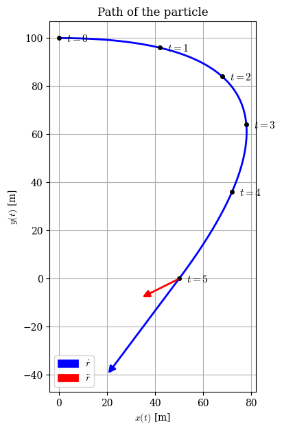
The curvilinear motion of a particle is defined by \(v_x = 50 - 16t\) m/s and \(y = 100 - 4t^2\) m, with \(x(0) = 0\). Plot the path of the particle and determine the velocity and acceleration when \(y = 0\).

Solution

We integrate \(v_x\) with the initial condition \(x(0) = 0\) to obtain \(x(t)\), then assemble the position vector and differentiate to get velocity and acceleration.

Code
import sympy as sp
from mechanicskit import la, ltx
t = sp.symbols('t', real=True, positive=True)
x = sp.Function('x')(t)
y_expr = 100 - 4*t**2

DE = sp.Eq(x.diff(t), 50 - 16*t)
ICs = {x.subs(t, 0): 0}
x_sol = sp.dsolve(DE, ics=ICs).rhs

ltx(r"x(t) &=", x_sol, r"\\ y(t) &=", y_expr, aligned=True)

\[ \begin{aligned}x(t) &=- 8 t^{2} + 50 t\\ y(t) &=100 - 4 t^{2}\end{aligned} \]

The particle reaches \(y = 0\) when

Code
t_y0 = sp.solve(sp.Eq(y_expr, 0), t)[0]
ltx(r"y = 0 \;\Rightarrow\; t =", t_y0, r"\text{ s}")

\[ y = 0 \;\Rightarrow\; t =5\text{ s} \]

Assembling the position vector and differentiating twice gives the velocity and acceleration.

Code
rr = sp.Matrix([x_sol, y_expr])
rr_dot = rr.diff(t)
rr_ddot = rr.diff(t, 2)

ltx(r"\bm r =", rr, r",\quad \dot{\bm r} =", rr_dot,
    r",\quad \ddot{\bm r} =", rr_ddot, arraystretch=1.5)

\[ {\def\arraystretch{1.5}\bm r =\left[\begin{matrix}- 8 t^{2} + 50 t\\100 - 4 t^{2}\end{matrix}\right],\quad \dot{\bm r} =\left[\begin{matrix}50 - 16 t\\- 8 t\end{matrix}\right],\quad \ddot{\bm r} =\left[\begin{matrix}-16\\-8\end{matrix}\right]} \]

Evaluating the velocity at \(t = 5\) s gives the answer. The acceleration is already constant.

Code
v_y0 = rr_dot.subs(t, t_y0)

ltx(r"\dot{\bm r}(5) =", v_y0, r"\text{ m/s},\quad \ddot{\bm r} =", rr_ddot,
    r"\text{ m/s}^2", arraystretch=1.5)

\[ {\def\arraystretch{1.5}\dot{\bm r}(5) =\left[\begin{matrix}-30\\-40\end{matrix}\right]\text{ m/s},\quad \ddot{\bm r} =\left[\begin{matrix}-16\\-8\end{matrix}\right]\text{ m/s}^2} \]

We plot the path with markers at integer seconds, and the velocity and acceleration vectors at \(y = 0\).

Code
from mechanicskit import fplot, arrow

t1 = float(t_y0)
pos = rr.subs(t, t_y0)

fig, ax = plt.subplots(figsize=(7, 7))
fplot(rr[0], rr[1], (t, 0, t1), ax=ax, color='b', linewidth=2)

for ti in range(6):
    p = rr.subs(t, ti)
    ax.plot(float(p[0]), float(p[1]), 'ko', markersize=4)
    ax.annotate(rf'$t={ti}$', (float(p[0]), float(p[1])),
                textcoords='offset points', xytext=(8, -4), fontsize=11)

arrow(pos, rr_dot.subs(t, t_y0), ax=ax, color='b', label=r'$\dot{r}$')
arrow(pos, rr_ddot, ax=ax, color='r', label=r'$\ddot{r}$')

ax.set_aspect('equal')
ax.set(xlabel=r'$x(t)$ [m]', ylabel=r'$y(t)$ [m]', title='Path of the particle')
ax.grid(True)
ax.legend(loc='lower left')
plt.show()

The acceleration is constant because \(v_x\) is linear in \(t\), which gives \(\ddot x = -16\), and \(y\) is quadratic in \(t\), which gives \(\ddot y = -8\).

Finally we animate the motion with the velocity and acceleration vectors attached to the moving particle.

Code
from matplotlib.animation import FuncAnimation
from mechanicskit import to_responsive_html

t1 = float(t_y0)
rr_n = sp.lambdify(t, rr, 'numpy')
rr_dot_n = sp.lambdify(t, rr_dot, 'numpy')
acc = np.array([float(rr_ddot[0]), float(rr_ddot[1])])

fig, ax = plt.subplots(figsize=(7, 7))
fplot(rr[0], rr[1], (t, 0, t1), ax=ax, color='0.7', linewidth=1.5)
ax.set_aspect('equal')
ax.set(xlim=(-25, 85), ylim=(-50, 110),
       xlabel=r'$x$ [m]', ylabel=r'$y$ [m]', title=f'Curvilinear motion, t=0')
ax.grid(True)

dot, = ax.plot([], [], 'ko', markersize=7)
v_arrow = arrow([0, 0], [1, 0], ax=ax, color='b', label=r'$\dot{r}$')
a_arrow = arrow([0, 0], [1, 0], ax=ax, color='r', label=r'$\ddot{r}$')
ax.legend(loc='lower left')

def update(frame):
    ti = t1 * frame / 59
    ax.set_title(f'Curvilinear motion, t={ti:.2f}')
    p = rr_n(ti).flatten()
    v = rr_dot_n(ti).flatten()
    dot.set_data([p[0]], [p[1]])
    v_arrow.set_positions((p[0], p[1]), (p[0]+v[0], p[1]+v[1]))
    a_arrow.set_positions((p[0], p[1]), (p[0]+acc[0], p[1]+acc[1]))
    return dot, v_arrow, a_arrow

anim = FuncAnimation(fig, update, frames=60, interval=50, blit=False)
plt.close(fig)
to_responsive_html(anim)

Example 9: Lead screw, 3D helical motion

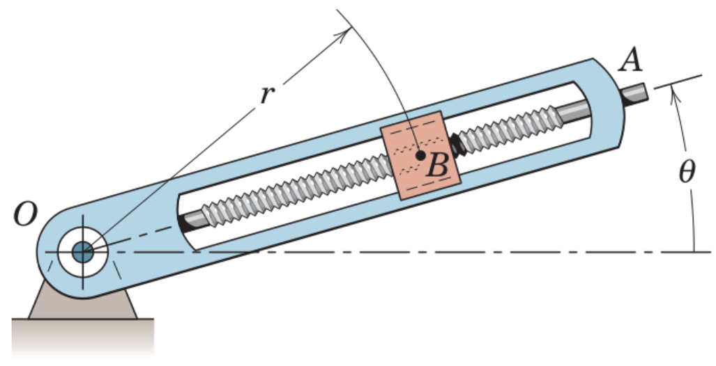
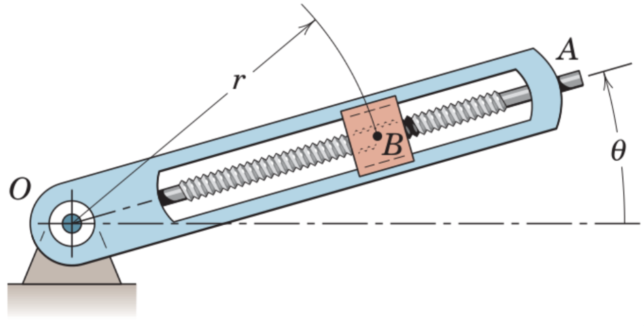
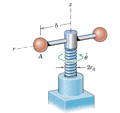
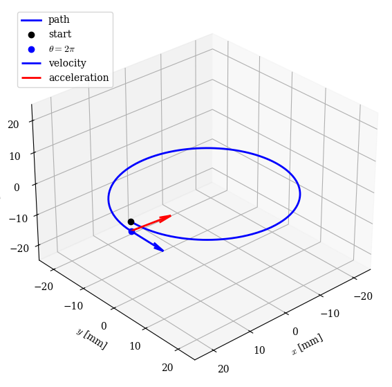
A power screw with lead \(L\) (the axial advancement per revolution) starts from rest and is rotated with an angular speed that increases uniformly with time, \(\dot\theta = k\,t\). The cross arm carries two balls at radial distance \(b\) from the screw axis. Determine the velocity and acceleration of the centre of ball \(A\) when the screw has turned through one complete revolution from rest, using \(k = 2\) rad/s\(^2\), \(b = 20\) mm, and \(L = 3\) mm.

Solution

The motion is a circular helix: ball \(A\) orbits the screw axis at constant radius \(b\) while the assembly descends along the axis at a rate proportional to the angular speed. We integrate the prescribed angular speed to obtain \(\theta(t)\), build the position vector in cylindrical form, and differentiate twice. Evaluating at the time when the screw has completed one full revolution yields the answer.

Code
import sympy as sp
from mechanicskit import la, ltx
t = sp.symbols('t', real=True, positive=True)

k, b, L = 2, 20, 3
theta_f = sp.Function('theta')(t)
DE = sp.Eq(theta_f.diff(t), k*t)
ICs = {theta_f.subs(t, 0): 0}
theta = sp.dsolve(DE, ics=ICs).rhs

ltx(r"\theta(t) =", theta)

\[ \theta(t) =t^{2} \]

The screw has completed one full revolution when \(\theta = 2\pi\), which fixes the time of interest.

Code
t_1 = sp.solve(sp.Eq(theta, 2*sp.pi), t)[0]
ltx(r"t_1 =", t_1, r"\;\text{s} \approx", float(t_1), r"\;\text{s}")

\[ t_1 =\sqrt{2} \sqrt{\pi}\;\text{s} \approx2.51\;\text{s} \]

The position vector of the ball centre superposes the circular motion of the cross arm onto the axial descent of the screw,

\[ \bm r(t) = \left[b\cos\theta,\; b\sin\theta,\; - \frac{L\,\theta}{2\pi}\right]^\mathsf T. \]

Differentiating twice with respect to time gives the velocity and acceleration.

Code
rr = sp.Matrix([b*sp.cos(theta), b*sp.sin(theta), -L*theta/(2*sp.pi)])
rr_dot = rr.diff(t)
rr_ddot = rr.diff(t, 2)

ltx(r"\bm r =", rr, r",\;\; \dot{\bm r} =", rr_dot,
    r",\;\; \ddot{\bm r} =", rr_ddot, arraystretch=1.5)

\[ {\def\arraystretch{1.5}\bm r =\left[\begin{matrix}20 \cos{\left(t^{2} \right)}\\20 \sin{\left(t^{2} \right)}\\- \dfrac{3 t^{2}}{2 \pi}\end{matrix}\right],\;\; \dot{\bm r} =\left[\begin{matrix}- 40 t \sin{\left(t^{2} \right)}\\40 t \cos{\left(t^{2} \right)}\\- \dfrac{3 t}{\pi}\end{matrix}\right],\;\; \ddot{\bm r} =\left[\begin{matrix}- 40 \left(2 t^{2} \cos{\left(t^{2} \right)} + \sin{\left(t^{2} \right)}\right)\\40 \left(- 2 t^{2} \sin{\left(t^{2} \right)} + \cos{\left(t^{2} \right)}\right)\\- \dfrac{3}{\pi}\end{matrix}\right]} \]

Substituting \(t_1\) delivers the position, velocity, and acceleration at the moment of one full revolution.

Code
p1 = rr.subs(t, t_1)
v1 = sp.simplify(rr_dot.subs(t, t_1))
a1 = sp.simplify(rr_ddot.subs(t, t_1))

ltx(r"\bm r(t_1) =", p1, r",\;\; \dot{\bm r}(t_1) =", v1,
    r",\;\; \ddot{\bm r}(t_1) =", a1, arraystretch=1.5)

\[ {\def\arraystretch{1.5}\bm r(t_1) =\left[\begin{matrix}20\\0\\-3\end{matrix}\right],\;\; \dot{\bm r}(t_1) =\left[\begin{matrix}0\\40 \sqrt{2} \sqrt{\pi}\\- \dfrac{3 \sqrt{2}}{\sqrt{\pi}}\end{matrix}\right],\;\; \ddot{\bm r}(t_1) =\left[\begin{matrix}- 160 \pi\\40\\- \dfrac{3}{\pi}\end{matrix}\right]} \]

Numerically the velocity and acceleration at \(t_1\) are

Code
import numpy as np
v1n = np.array(v1, dtype=float).flatten()
a1n = np.array(a1, dtype=float).flatten()

ltx(r"\dot{\bm r}(t_1) \approx", v1n.reshape(3, 1),
    r"\;\text{mm/s},\quad \ddot{\bm r}(t_1) \approx",
    a1n.reshape(3, 1), r"\;\text{mm/s}^2", arraystretch=1.5)

\[ {\def\arraystretch{1.5}\dot{\bm r}(t_1) \approx\begin{bmatrix}0.00 \\ 100.27 \\ -2.39\end{bmatrix}\;\text{mm/s},\quad \ddot{\bm r}(t_1) \approx\begin{bmatrix}-502.65 \\ 40.00 \\ -0.95\end{bmatrix}\;\text{mm/s}^2} \]

Two observations stand out. The horizontal velocity component points purely in the \(y\) direction because after a full revolution \(\theta = 2\pi\) places ball \(A\) back on the \(+x\) axis, where the tangent to the circle is along \(\bm j\). The acceleration is dominated by the centripetal term \(b\,\dot\theta^2\) in the \(-x\) direction, which at \(t_1\) equals \(b\,(2t_1)^2 = 8\pi b \approx 503\) mm/s\(^2\) and dwarfs the tangential and axial contributions.

We visualise the helical path from start to one full revolution, with the velocity and acceleration vectors attached at \(t_1\).

Code
import matplotlib.pyplot as plt

rr_n = sp.lambdify(t, rr, 'numpy')
rr_dot_n = sp.lambdify(t, rr_dot, 'numpy')
rr_ddot_n = sp.lambdify(t, rr_ddot, 'numpy')

t_vals = np.linspace(0, float(t_1), 200)
path = np.array([rr_n(ti).flatten() for ti in t_vals])
p1n = rr_n(float(t_1)).flatten()

fig = plt.figure(figsize=(8, 7))
ax = fig.add_subplot(111, projection='3d')
ax.plot(path[:, 0], path[:, 1], path[:, 2], 'b-', linewidth=2, label='path')
ax.plot([b], [0], [0], 'ko', markersize=6, label='start')
ax.plot([p1n[0]], [p1n[1]], [p1n[2]], 'bo', markersize=6,
        label=r'$\theta = 2\pi$')

ax.quiver(*p1n, *(v1n*0.1), color='b', linewidth=2, label='velocity')
ax.quiver(*p1n, *(a1n*0.02), color='r', linewidth=2, label='acceleration')

ax.set(xlabel=r'$x$ [mm]', ylabel=r'$y$ [mm]', zlabel=r'$z$ [mm]')
ax.set_xlim(-25, 25); ax.set_ylim(-25, 25); ax.set_zlim(-25, 25)
ax.view_init(elev=30, azim=48)
ax.legend(loc='upper left')
plt.show()

We extend the simulation to ten full revolutions to expose the helical structure of the trajectory and animate the velocity and acceleration vectors as they sweep around the screw axis.

Code
from matplotlib.animation import FuncAnimation, FFMpegWriter

t_end = float(sp.solve(sp.Eq(theta, 20*sp.pi), t)[0])
t_anim = np.linspace(0, t_end, 600)
path_long = np.array([rr_n(ti).flatten() for ti in t_anim])

fig = plt.figure(figsize=(8, 7))
ax = fig.add_subplot(111, projection='3d')
ax.plot(path_long[:, 0], path_long[:, 1], path_long[:, 2],
        color='0.7', linewidth=1.0)
zmin = float(path_long[:, 2].min()) - 2
ax.set(xlabel=r'$x$ [mm]', ylabel=r'$y$ [mm]', zlabel=r'$z$ [mm]')
ax.set_xlim(-25, 25); ax.set_ylim(-25, 25); ax.set_zlim(zmin, 2)
ax.view_init(elev=25, azim=48)

dot, = ax.plot([], [], [], 'ko', markersize=6)
quivers = {'v': ax.quiver(0, 0, 0, 0, 0, 0, color='b', linewidth=2),
           'a': ax.quiver(0, 0, 0, 0, 0, 0, color='r', linewidth=2)}
title = ax.set_title('')

frames = 300
def update(frame):
    ti = t_end * frame / (frames - 1)
    p = rr_n(ti).flatten()
    v = rr_dot_n(ti).flatten()
    a = rr_ddot_n(ti).flatten()
    dot.set_data([p[0]], [p[1]])
    dot.set_3d_properties([p[2]])
    quivers['v'].remove()
    quivers['a'].remove()
    quivers['v'] = ax.quiver(*p, *(v*0.02), color='b', linewidth=2)
    quivers['a'] = ax.quiver(*p, *(a*0.004), color='r', linewidth=2)
    title.set_text(rf'$t = {ti:.2f}$ s, $\theta = {float(theta.subs(t, ti)):.2f}$ rad')
    return dot, quivers['v'], quivers['a'], title

anim = FuncAnimation(fig, update, frames=frames, interval=50, blit=False)
anim.save('graphics/kinematics_lead_screw.mp4', writer=FFMpegWriter(fps=30))
plt.close(fig)

Example 10: Tractor hoisting, constrained motion

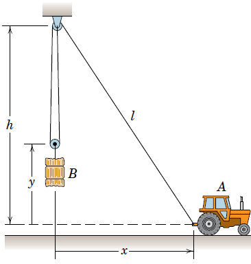
A tractor at \(A\) moves horizontally with forward velocity \(v_A\) and hoists a bale \(B\) via a rope routed over a fixed pulley at \(C\), which sits at height \(h\) above the ground. The rope passes from the tractor up to the top pulley, descends to a movable pulley fastened to the bale, and returns to a fixed anchor at the same height. The bale rises along a vertical line directly below \(C\). Determine the upward velocity \(v_B\) of the bale as a function of \(v_A\) and the tractor position \(x\).

Solution

The kinematic relation between the two velocities follows entirely from geometry and the inextensibility of the rope. Two constraints capture the setup. The right triangle formed by the tractor, the pulley, and the ground gives

\[ x^2 + h^2 = l^2, \]

where \(l\) is the slanted rope segment from \(A\) to \(C\). The total rope length \(L\) is fixed,

\[ L = 2(h - y) + l, \]

since the rope between the top pulley and the bale comprises two parallel segments of length \(h - y\). Differentiating both constraints with respect to time and solving the resulting linear pair for \(v_B\) delivers the answer.

Code
import sympy as sp
from mechanicskit import la, ltx
t = sp.symbols('t', real=True, positive=True)
h, L = sp.symbols('h L', positive=True)
v_A, v_B, l_dot = sp.symbols('v_A v_B l_dot', real=True)
x_t = sp.Function('x')(t)
y_t = sp.Function('y')(t)
l_t = sp.Function('l')(t)

c1 = sp.Eq(x_t**2 + h**2, l_t**2)
c2 = sp.Eq(L, 2*(h - y_t) + l_t)

ltx(r"\text{(geometry)}\quad ", c1, r",\quad \text{(rope)}\quad ", c2)

\[ \text{(geometry)}\quad h^{2} + x^{2}{\left(t \right)} = l^{2}{\left(t \right)},\quad \text{(rope)}\quad L = 2 h + l{\left(t \right)} - 2 y{\left(t \right)} \]

Differentiating each constraint with respect to \(t\) and replacing \(\dot x\), \(\dot y\), \(\dot l\) with the named velocities \(v_A\), \(v_B\), \(\dot l\) produces a linear system in the rate variables.

Code
subs = {x_t.diff(t): v_A, y_t.diff(t): v_B, l_t.diff(t): l_dot}
c1_dot = sp.Eq(c1.lhs.diff(t), c1.rhs.diff(t)).subs(subs)
c2_dot = sp.Eq(c2.lhs.diff(t), c2.rhs.diff(t)).subs(subs)

ltx(c1_dot, r",\quad", c2_dot)

\[ 2 v_{A} x{\left(t \right)} = 2 l_{dot} l{\left(t \right)},\quad0 = l_{dot} - 2 v_{B} \]

We solve the system for \(v_B\) and \(\dot l\), then eliminate \(l\) in favour of \(x\) using \(l = \sqrt{x^2 + h^2}\).

Code
x = sp.symbols('x', positive=True)
sol = sp.solve([c1_dot, c2_dot], [v_B, l_dot])
v_B_expr = sp.simplify(sol[v_B].subs(l_t, sp.sqrt(x**2 + h**2)).subs(x_t, x))
y_expr = sp.solve(c2.subs(l_t, sp.sqrt(x**2 + h**2)), y_t)[0]

ltx(r"v_B =", v_B_expr, r",\quad y(x) =", y_expr)

\[ v_B =\dfrac{v_{A} x}{2 \sqrt{h^{2} + x^{2}}},\quad y(x) =- \dfrac{L}{2} + h + \dfrac{\sqrt{h^{2} + x^{2}}}{2} \]

The bale velocity vanishes at \(x = 0\) and approaches \(v_A/2\) as \(x \to \infty\), since the rope segment \(l\) then aligns with the horizontal and the tractor essentially reels in rope at its own speed, with the factor of one half coming from the two-to-one mechanical advantage of the movable pulley.

For the numerical case we take \(h = 5\) m and a rope length \(L = 3h = 15\) m, so that the bale rests on the ground when the tractor sits beneath the pulley. The tractor advances until the bale reaches a height of \(y = 4\) m, which by inversion of \(y(x)\) corresponds to a tractor position \(x = 12\) m.

Code
params = {h: 5, L: 15}
y_x = y_expr.subs(params)
v_B_over_v_A = (v_B_expr/v_A).subs(params)
x_final = sp.solve(sp.Eq(y_x, 4), x)[0]

ltx(r"y(x) =", y_x, r",\quad \frac{v_B}{v_A} =", v_B_over_v_A,
    r",\quad x|_{y=4} =", x_final)

\[ y(x) =\dfrac{\sqrt{x^{2} + 25}}{2} - \dfrac{5}{2},\quad \frac{v_B}{v_A} =\dfrac{x}{2 \sqrt{x^{2} + 25}},\quad x|_{y=4} =12 \]

We sketch the geometry at \(x = 4\) m, drawing the two rope segments from the tractor to the top pulley and from the pulley down to the bale.

Code
import numpy as np
import matplotlib.pyplot as plt

y_n = sp.lambdify(x, y_x, 'numpy')
x_i = 4.0
A_i = np.array([x_i, 0.0])
B_i = np.array([0.0, float(y_n(x_i))])
C = np.array([0.0, 5.0])

fig, ax = plt.subplots(figsize=(8, 4))
ax.plot([C[0], A_i[0]], [C[1], A_i[1]], '-ko', markerfacecolor='k', linewidth=2)
ax.plot([C[0], B_i[0]], [C[1], B_i[1]], '-ko', markerfacecolor='k', linewidth=2)
ax.plot([0, 15], [0, 0], 'k-', linewidth=0.8)
ax.annotate(r'$A$', A_i, xytext=(8, 8), textcoords='offset points', fontsize=12)
ax.annotate(r'$B$', B_i, xytext=(8, 8), textcoords='offset points', fontsize=12)
ax.annotate(r'$C$', C,   xytext=(8, 8), textcoords='offset points', fontsize=12)
ax.set_aspect('equal')
ax.set(xlim=(-1, 15), ylim=(-0.5, 6.5),
       xlabel=r'$x$ [m]', ylabel=r'$y$ [m]')
ax.grid(True)
plt.show()

Animating \(x\) from \(0\) to \(12\) m shows how the bale climbs and the rope geometry evolves. The animation is exported to mp4 and embedded below.

Code
from matplotlib.animation import FuncAnimation, FFMpegWriter

fig, ax = plt.subplots(figsize=(8, 4))
ax.plot([0, 15], [0, 0], 'k-', linewidth=0.8)
line_AC, = ax.plot([], [], '-ko', markerfacecolor='k', linewidth=2)
line_BC, = ax.plot([], [], '-ko', markerfacecolor='k', linewidth=2)
ax.plot(*C, 'ko', markerfacecolor='k')
txt_A = ax.text(0, 0, r'$A$', fontsize=12)
txt_B = ax.text(0, 0, r'$B$', fontsize=12)
ax.text(C[0]+0.2, C[1]+0.2, r'$C$', fontsize=12)
ax.set_aspect('equal')
ax.set(xlim=(-1, 15), ylim=(-0.5, 6.5),
       xlabel=r'$x$ [m]', ylabel=r'$y$ [m]')
ax.grid(True)
title = ax.set_title('')

frames = 150
x_path = np.linspace(0, float(x_final), frames)

def update(frame):
    xi = x_path[frame]
    A = np.array([xi, 0.0])
    B = np.array([0.0, float(y_n(xi))])
    line_AC.set_data([C[0], A[0]], [C[1], A[1]])
    line_BC.set_data([C[0], B[0]], [C[1], B[1]])
    txt_A.set_position((A[0]+0.2, A[1]+0.2))
    txt_B.set_position((B[0]+0.2, B[1]+0.2))
    title.set_text(rf'$x = {xi:.2f}$ m, $y = {B[1]:.2f}$ m')
    return line_AC, line_BC, txt_A, txt_B, title

anim = FuncAnimation(fig, update, frames=frames, interval=50, blit=False)
anim.save('graphics/kinematics_tractor_hoist.mp4', writer=FFMpegWriter(fps=30))
plt.close(fig)

Example 11: Crank-slider mechanism

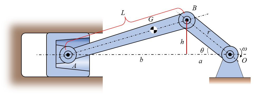
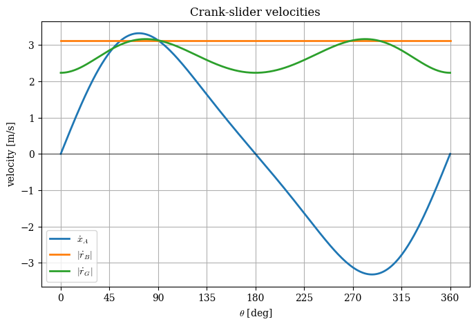
Study the motion of a slider-crank mechanism running at constant angular velocity \(\omega = 25\) rad/s. The crank has length \(r = 125\) mm and the connecting rod has length \(L = 350\) mm. The centre of mass \(G\) of the connecting rod sits \(100\) mm from the crank pin \(B\) along the rod, so \(250\) mm from the slider pin \(A\). Determine the velocity and acceleration of points \(A\), \(B\), and \(G\) as functions of the crank angle \(\theta\), and plot their magnitudes over a full revolution.

Solution

We place the crank pivot \(O\) at the origin and let the slider \(A\) travel along the negative \(x\)-axis. With the crank angle \(\theta\) measured from the horizontal, the crank pin sits at

\[ \bm r_B = r\bigl(-\cos\theta,\; \sin\theta\bigr). \]

The slider pin lies on the \(x\)-axis at horizontal distance \(a + b\) from \(O\), where \(a = r\cos\theta\) is the horizontal projection of the crank and \(b = \sqrt{L^2 - h^2}\) comes from Pythagoras applied to the connecting rod with \(h = r\sin\theta\). Hence

\[ \bm r_A = \bigl(-(a + b),\; 0\bigr). \]

The centre of mass \(G\) partitions the rod with \(BG = 100\) mm out of \(L = 350\) mm, so

\[ \bm r_G = \bm r_B + \frac{BG}{L}\bigl(\bm r_A - \bm r_B\bigr). \]

Since \(\theta = \omega t\) with \(\dot\theta = \omega\) constant and \(\ddot\theta = 0\), time derivatives reduce to derivatives with respect to \(\theta\),

\[ \dot{\bm r} = \omega\,\frac{\mathrm d \bm r}{\mathrm d \theta}, \qquad \ddot{\bm r} = \omega^2\,\frac{\mathrm d^2 \bm r}{\mathrm d \theta^2}, \]

which lets us treat \(\theta\) as the independent variable throughout.

Code
import sympy as sp
from mechanicskit import la, ltx
theta, omega = sp.symbols('theta omega', positive=True)
r, L, BG = sp.Rational(125, 1000), sp.Rational(350, 1000), sp.Rational(100, 1000)
omega_val = 25

a = r*sp.cos(theta)
h = r*sp.sin(theta)
b = sp.sqrt(L**2 - h**2)

rr_B = sp.Matrix([-r*sp.cos(theta), r*sp.sin(theta)])
rr_A = sp.Matrix([-(a + b), 0])
rr_G = sp.simplify(rr_B + (BG/L)*(rr_A - rr_B))

ltx(r"\bm r_A &=", rr_A, r",\\[1em]  \bm r_B &=", rr_B,
    r",\\[1em] \bm r_G &=", rr_G, aligned=True,arraystretch=1.5)

\[ {\def\arraystretch{1.5}\begin{aligned}\bm r_A &=\left[\begin{matrix}- \sqrt{\dfrac{49}{400} - \dfrac{\sin^{2}{\left(\theta \right)}}{64}} - \dfrac{\cos{\left(\theta \right)}}{8}\\0\end{matrix}\right],\\[1em] \bm r_B &=\left[\begin{matrix}- \dfrac{\cos{\left(\theta \right)}}{8}\\\dfrac{\sin{\left(\theta \right)}}{8}\end{matrix}\right],\\[1em] \bm r_G &=\left[\begin{matrix}- \dfrac{\sqrt{196 - 25 \sin^{2}{\left(\theta \right)}}}{140} - \dfrac{\cos{\left(\theta \right)}}{8}\\\dfrac{5 \sin{\left(\theta \right)}}{56}\end{matrix}\right]\end{aligned}} \]

Differentiating each position with respect to \(\theta\) (and multiplying by \(\omega\) or \(\omega^2\) for the time derivatives) gives the velocity and acceleration. The crank pin moves on a circle, so \(|\dot{\bm r}_B| = r\omega\) and \(|\ddot{\bm r}_B| = r\omega^2\) are constants. The slider velocity vanishes twice per revolution, at the dead-centre positions \(\theta = 0\) and \(\theta = \pi\), which forces large slider accelerations near those angles.

Code
def deriv(rr):
    return omega*rr.diff(theta), omega**2*rr.diff(theta, 2)

rr_A_dot, rr_A_ddot = deriv(rr_A)
rr_B_dot, rr_B_ddot = deriv(rr_B)
rr_G_dot, rr_G_ddot = deriv(rr_G)

Substituting \(\omega = 25\) rad/s, we plot the slider velocity \(\dot x_A\) alongside the magnitudes \(|\dot{\bm r}_B|\) and \(|\dot{\bm r}_G|\). The crank pin runs at the constant \(|\dot{\bm r}_B| = r\omega \approx 3.13\) m/s, while the slider velocity oscillates between \(\pm\) a peak just above \(r\omega\) and vanishes at the dead-centre positions \(\theta = 0\) and \(\theta = \pi\).

Code
import numpy as np
import matplotlib.pyplot as plt

vAx_n = sp.lambdify(theta, rr_A_dot[0].subs(omega, omega_val), 'numpy')
vB_mag = sp.sqrt(rr_B_dot.dot(rr_B_dot)).subs(omega, omega_val)
vG_mag = sp.sqrt(rr_G_dot.dot(rr_G_dot)).subs(omega, omega_val)
vB_n = sp.lambdify(theta, vB_mag, 'numpy')
vG_n = sp.lambdify(theta, vG_mag, 'numpy')

th = np.linspace(0, 2*np.pi, 400)
deg = np.degrees(th)
fig, ax = plt.subplots(figsize=(8, 5))
ax.plot(deg, vAx_n(th), color='C0', label=r'$\dot{x}_A$', linewidth=2)
ax.plot(deg, np.full_like(th, float(vB_n(0))), color='C1',
        label=r'$|\dot{r}_B|$', linewidth=2)
ax.plot(deg, vG_n(th), color='C2', label=r'$|\dot{r}_G|$', linewidth=2)
ax.axhline(0, color='k', linewidth=0.5)
ax.set(xlabel=r'$\theta$ [deg]', ylabel='velocity [m/s]',
       title='Crank-slider velocities')
ax.set_xticks(range(0, 361, 45))
ax.grid(True); ax.legend(loc='lower left')
plt.show()

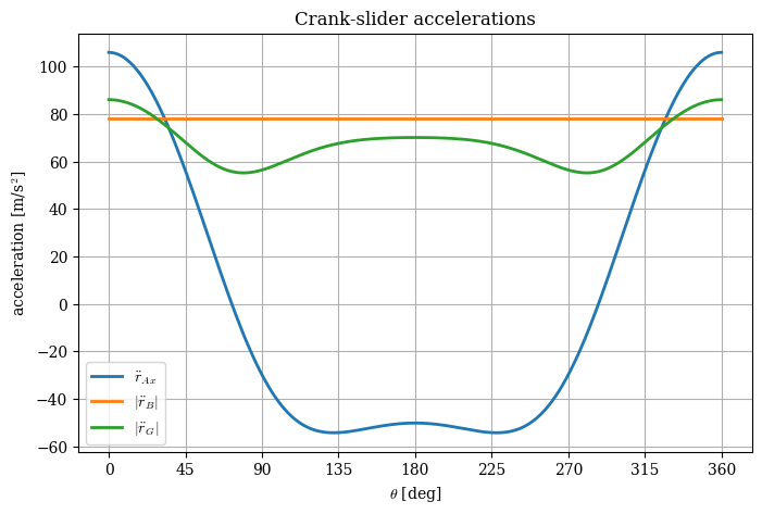
The acceleration plot reveals the asymmetry inherent to a finite connecting rod: the slider acceleration \(\ddot r_{Ax}\) swings between large positive values near top dead centre and smaller negative values around bottom dead centre, while \(|\ddot{\bm r}_B| = r\omega^2 \approx 78.1\) m/s\(^2\) remains constant.

Code
aAx = rr_A_ddot[0].subs(omega, omega_val)
aB_mag = sp.sqrt(rr_B_ddot.dot(rr_B_ddot)).subs(omega, omega_val)
aG_mag = sp.sqrt(rr_G_ddot.dot(rr_G_ddot)).subs(omega, omega_val)

aAx_n = sp.lambdify(theta, aAx, 'numpy')
aB_n = sp.lambdify(theta, aB_mag, 'numpy')
aG_n = sp.lambdify(theta, aG_mag, 'numpy')

fig, ax = plt.subplots(figsize=(8, 5))
ax.plot(np.degrees(th), aAx_n(th), label=r'$\ddot{r}_{Ax}$', linewidth=2)
ax.plot(np.degrees(th), np.full_like(th, aB_n(0)),
        label=r'$|\ddot{r}_B|$', linewidth=2)
ax.plot(np.degrees(th), aG_n(th), label=r'$|\ddot{r}_G|$', linewidth=2)
ax.set(xlabel=r'$\theta$ [deg]', ylabel=r'acceleration [m/s$^2$]',
       title='Crank-slider accelerations')
ax.set_xticks(range(0, 361, 45))
ax.grid(True); ax.legend(loc='lower left')
plt.show()

Finally we animate one full revolution as a synchronised triple view: the mechanism on the left with velocity (blue) and acceleration (red) arrows attached to \(A\), \(B\), and \(G\), the speed plot in the upper right with markers tracking the current angle, and the acceleration plot in the lower right with the same. The animation is rendered to mp4 at 60 fps and embedded below.

Code
from matplotlib.animation import FuncAnimation, FFMpegWriter
from mechanicskit import arrow

rr_A_n = sp.lambdify(theta, rr_A, 'numpy')
rr_B_n = sp.lambdify(theta, rr_B, 'numpy')
rr_G_n = sp.lambdify(theta, rr_G, 'numpy')

vA_v = sp.lambdify(theta, rr_A_dot.subs(omega, omega_val), 'numpy')
vB_v = sp.lambdify(theta, rr_B_dot.subs(omega, omega_val), 'numpy')
vG_v = sp.lambdify(theta, rr_G_dot.subs(omega, omega_val), 'numpy')
aA_v = sp.lambdify(theta, rr_A_ddot.subs(omega, omega_val), 'numpy')
aB_v = sp.lambdify(theta, rr_B_ddot.subs(omega, omega_val), 'numpy')
aG_v = sp.lambdify(theta, rr_G_ddot.subs(omega, omega_val), 'numpy')

th_curve = np.linspace(0, 2*np.pi, 400)
deg_curve = np.degrees(th_curve)
vAx_curve = vAx_n(th_curve)
vB_curve = np.full_like(th_curve, float(vB_n(0)))
vG_curve = vG_n(th_curve)
aA_curve = aAx_n(th_curve)
aB_curve = np.full_like(th_curve, float(aB_n(0)))
aG_curve = aG_n(th_curve)

fig = plt.figure(figsize=(14, 7))
gs = fig.add_gridspec(2, 2, width_ratios=[1.6, 1])
ax_mech = fig.add_subplot(gs[:, 0])
ax_v = fig.add_subplot(gs[0, 1])
ax_a = fig.add_subplot(gs[1, 1])

ax_mech.plot(0, 0, 'ks', markersize=8)
ax_mech.text(0.005, -0.04, r'$O$', fontsize=12)
crank, = ax_mech.plot([], [], '-o', color='C0', markerfacecolor='C0',
                     markersize=8, linewidth=3)
rod, = ax_mech.plot([], [], '-o', color='C1', markerfacecolor='C1',
                   markersize=8, linewidth=3)
slider, = ax_mech.plot([], [], 's', color='k', markerfacecolor='0.7',
                      markersize=18)
gpoint, = ax_mech.plot([], [], 'o', color='C3', markerfacecolor='C3',
                      markersize=10)
txt_A = ax_mech.text(0, 0, r'$A$', fontsize=12)
txt_B = ax_mech.text(0, 0, r'$B$', fontsize=12)
txt_G = ax_mech.text(0, 0, r'$G$', fontsize=12)

vs, as_ = 0.04, 0.001
v_arr = {pt: arrow([0, 0], [1e-3, 0], ax=ax_mech, color='b', linewidth=2)
         for pt in 'ABG'}
a_arr = {pt: arrow([0, 0], [1e-3, 0], ax=ax_mech, color='r', linewidth=2)
         for pt in 'ABG'}

ax_mech.set_aspect('equal')
ax_mech.set(xlim=(-0.6, 0.2), ylim=(-0.22, 0.22),
           xlabel=r'$x$ [m]', ylabel=r'$y$ [m]',
           title=f'$\\theta=0^\\circ$')
ax_mech.grid(True)

ax_v.plot(deg_curve, vAx_curve, color='C0', label=r'$\dot{x}_A$', linewidth=1.5)
ax_v.plot(deg_curve, vB_curve, color='C1', label=r'$|\dot{r}_B|$', linewidth=1.5)
ax_v.plot(deg_curve, vG_curve, color='C2', label=r'$|\dot{r}_G|$', linewidth=1.5)
ax_v.axhline(0, color='k', linewidth=0.5)
mvA, = ax_v.plot([], [], 'o', color='C0', markersize=8)
mvB, = ax_v.plot([], [], 'o', color='C1', markersize=8)
mvG, = ax_v.plot([], [], 'o', color='C2', markersize=8)
ax_v.set(xlabel=r'$\theta$ [deg]', ylabel='velocity [m/s]', xlim=(0, 360))
ax_v.set_xticks(range(0, 361, 90))
ax_v.grid(True); ax_v.legend(loc='lower left')

ax_a.plot(deg_curve, aA_curve, color='C0', label=r'$\ddot{r}_{Ax}$', linewidth=1.5)
ax_a.plot(deg_curve, aB_curve, color='C1', label=r'$|\ddot{r}_B|$', linewidth=1.5)
ax_a.plot(deg_curve, aG_curve, color='C2', label=r'$|\ddot{r}_G|$', linewidth=1.5)
maA, = ax_a.plot([], [], 'o', color='C0', markersize=8)
maB, = ax_a.plot([], [], 'o', color='C1', markersize=8)
maG, = ax_a.plot([], [], 'o', color='C2', markersize=8)
ax_a.set(xlabel=r'$\theta$ [deg]', ylabel=r'accel [m/s$^2$]', xlim=(0, 360))
ax_a.set_xticks(range(0, 361, 90))
ax_a.grid(True); ax_a.legend(loc='lower left')
fig.tight_layout()

frames = 240
def update(frame):
    th_i = 2*np.pi * frame / (frames - 1)
    ax_mech.set_title(f'$\\theta=${int(np.degrees(th_i))}$^\\circ$')
    deg_i = np.degrees(th_i)
    A = rr_A_n(th_i).flatten()
    B = rr_B_n(th_i).flatten()
    G = rr_G_n(th_i).flatten()
    pts = {'A': A, 'B': B, 'G': G}
    vels = {'A': np.array(vA_v(th_i), dtype=float).flatten(),
            'B': np.array(vB_v(th_i), dtype=float).flatten(),
            'G': np.array(vG_v(th_i), dtype=float).flatten()}
    accs = {'A': np.array(aA_v(th_i), dtype=float).flatten(),
            'B': np.array(aB_v(th_i), dtype=float).flatten(),
            'G': np.array(aG_v(th_i), dtype=float).flatten()}

    crank.set_data([0, B[0]], [0, B[1]])
    rod.set_data([B[0], A[0]], [B[1], A[1]])
    slider.set_data([A[0]], [A[1]])
    gpoint.set_data([G[0]], [G[1]])
    txt_A.set_position((A[0]-0.015, A[1]+0.025))
    txt_B.set_position((B[0]+0.005, B[1]+0.020))
    txt_G.set_position((G[0]+0.005, G[1]+0.020))

    for pt in 'ABG':
        p = pts[pt]; v = vels[pt]; a = accs[pt]
        v_arr[pt].set_positions((p[0], p[1]),
                                (p[0]+v[0]*vs, p[1]+v[1]*vs))
        a_arr[pt].set_positions((p[0], p[1]),
                                (p[0]+a[0]*as_, p[1]+a[1]*as_))

    mvA.set_data([deg_i], [vels['A'][0]])
    mvB.set_data([deg_i], [np.linalg.norm(vels['B'])])
    mvG.set_data([deg_i], [np.linalg.norm(vels['G'])])
    maA.set_data([deg_i], [accs['A'][0]])
    maB.set_data([deg_i], [np.linalg.norm(accs['B'])])
    maG.set_data([deg_i], [np.linalg.norm(accs['G'])])
    return ()

anim = FuncAnimation(fig, update, frames=frames, interval=1000/60, blit=False)
anim.save('graphics/kinematics_crank_slider.mp4',
          writer=FFMpegWriter(fps=60))
plt.close(fig)

Three features of the animation deserve comment. The slider velocity and acceleration run out of phase. At the dead-centre positions \(\theta = 0\) and \(\theta = \pi\) the velocity \(\dot x_A\) vanishes, yet the acceleration \(\ddot r_{Ax}\) takes its largest values there. Conversely, where \(\dot x_A\) peaks, \(\ddot r_{Ax}\) has already crossed zero. The relationship is not the rigid quarter-period offset of simple harmonic motion, since the finite connecting rod skews both curves.

The velocity and acceleration at \(G\) are not always perpendicular to one another. The crank pin \(B\) travels on a circle, so its acceleration is purely centripetal and orthogonal to the tangential velocity at every instant. The point \(G\) traces a more complicated curve, and its acceleration carries components both along and across the velocity direction, which the animation makes visible as the blue and red arrows at \(G\) rarely meet at right angles.

Finally, \(\ddot r_{Ax}\) vanishes at the angles where the acceleration vectors at \(B\) and \(G\) stand vertical. The slider can only be accelerated through the horizontal projection of the pin accelerations transmitted by the connecting rod. When that projection cancels, the rod imparts no horizontal impulse to \(A\), and the slider coasts at its peak speed.