6.4  Rigid Body Kinematics

Absolute Motion

The absolute approach to plane motion writes the position of every point as an explicit function of time, then differentiates to obtain velocity and acceleration. It is mechanical and always works, but the algebra grows quickly with the number of links. We use the rolling wheel as a worked example before moving on to a more efficient approach in the next section.

Wheel rolling without slipping

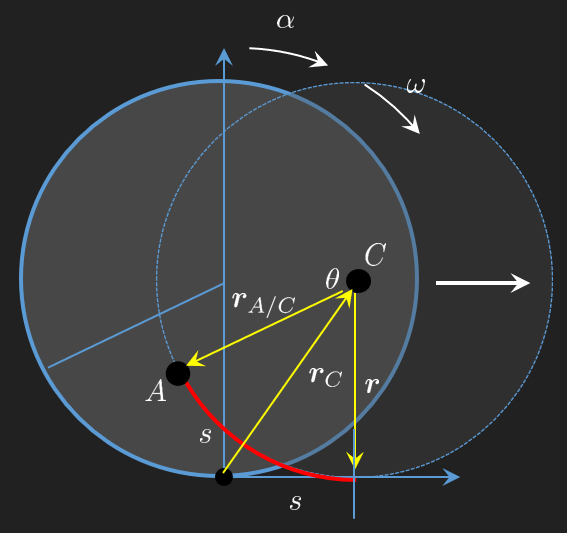
Rolling wheel kinematics

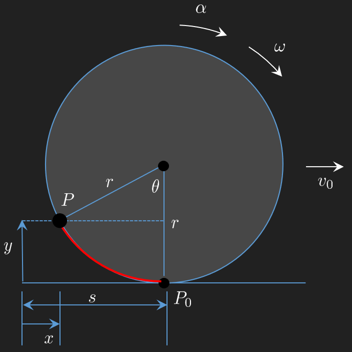
The marked point \(P\) on the rim traces a cycloid as the wheel rolls. Reading its coordinates off the figure,

\[ \begin{aligned} & x = s - r \sin\theta \\ & y = r - r \cos\theta \end{aligned} \]

where \(s\) is the horizontal travel of the centre and \(\theta\) the rotation angle.

Rolling without slipping ties the translation of the centre to the rotation of the wheel through \(s = r\theta\), so

\[ x = r\theta - r \sin\theta \]

Differentiating the rolling constraint with respect to time gives the translational velocity and acceleration of the centre,

\[ \begin{aligned} & v_0 = r \omega \\ & a_0 = r \alpha = r \dot\omega = r \ddot\theta \end{aligned} \]

Substituting \(s(t) = r\theta(t)\) gives the position of \(P\) as a function of time,

\[ P\left\{\begin{array}{l} x(t) = r(\theta(t) - \sin\theta(t)) \\ y(t) = r(1 - \cos\theta(t)) \end{array}\right. \]

Since the centre moves rectilinearly, its speed \(v_0\) coincides with the overall speed \(v\) and its acceleration \(a_0\) with the tangential component \(a_t\). Inverting the rolling relations then expresses the angular quantities in terms of linear ones,

\[ \begin{aligned} & \omega = \frac{v}{r} \\ & \alpha = \frac{a_t}{r} \end{aligned} \]

Putting everything together, the cycloid and its time derivatives read

\[ \begin{aligned} & P=\left\{\begin{array}{l} x(t) = r\theta - r \sin\theta \\ y(t) = r - r \cos\theta \end{array}\right. \\ & \dot P=\left\{\begin{array}{l} \dot x(t) = r\omega(1 - \cos\theta) = v_0(1 - \cos\theta) \\ \dot y(t) = r\omega \sin\theta = v_0 \sin\theta \end{array}\right. \\ & \ddot P=\left\{\begin{array}{l} \ddot x(t) = r\alpha(1 - \cos\theta) + r\omega^2 \sin\theta = a_0(1 - \cos\theta) + \omega v_0 \sin\theta \\ \ddot y(t) = r\alpha \sin\theta + r\omega^2 \cos\theta = a_0 \sin\theta + \omega v_0 \cos\theta \end{array}\right. \end{aligned} \]

Cycloid path

The recipe is mechanical: write the position vector as a function of time, differentiate twice, and use the rolling constraint to eliminate intermediate variables. It always works, but it is often laborious. In what follows we develop a more direct approach based on angular velocity and acceleration vectors.

Example - Window

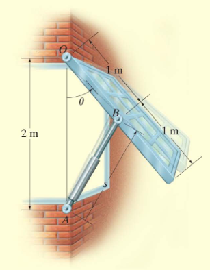
Window opened by a hydraulic piston

A window is held by a pin at \(O\) and opened by a hydraulic piston anchored at \(A\) on the wall, 2 m below \(O\), and attached to the window at \(B\), 1 m from the hinge. The piston extends at a constant rate \(\dot s = 300\) mm/s. We want to know

  • the maximum opening angle of the window,
  • the angular velocity \(\dot\theta\) and the peripheral speed at the bottom edge of the window as functions of \(\theta\),
  • the angular acceleration \(\ddot\theta\) and whether the window speeds up or slows down as it opens.

Solution

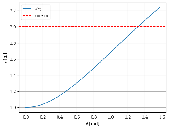
We place the origin at the upper hinge \(O\) and let \(\theta\) be the angle between the arm \(OB\) and the downward vertical. From the figure,

\[ \bm r_{OA} = \begin{bmatrix}0\\-2\end{bmatrix} \text{ m}, \qquad \bm r_{OB}(\theta) = \begin{bmatrix}\sin\theta\\-\cos\theta\end{bmatrix} \text{ m} \]

The piston vector connects \(A\) to \(B\) and its length is the piston stroke \(s\).

Code
import sympy as sp
from mechanicskit import la, ltx, fplot
import matplotlib.pyplot as plt
import numpy as np

theta = sp.symbols('theta', real=True, positive=True)

rr_OA = sp.Matrix([0, -2])
rr_OB = sp.Matrix([sp.sin(theta), -sp.cos(theta)])
rr_AB = rr_OB - rr_OA

s = sp.sqrt(rr_AB.dot(rr_AB))
s = sp.simplify(s)

ltx(r"\bm r_{AB} =", rr_AB, r",\qquad s(\theta) =", s)

\[ \bm r_{AB} =\left[\begin{matrix}\sin{\left(\theta \right)}\\2 - \cos{\left(\theta \right)}\end{matrix}\right],\qquad s(\theta) =\sqrt{5 - 4 \cos{\left(\theta \right)}} \]

Maximum opening angle

The piston is fully extended when \(s = 2\) m. Plotting \(s(\theta)\) lets us read off the angle where this happens, and solving the equation gives the exact value.

Code
import sympy as sp
fig, ax = plt.subplots()
fplot(s, (theta, 0, sp.pi/2), ax=ax, label=r'$s(\theta)$')
ax.axhline(2, color='r', linestyle='--', label=r'$s = 2$ m')
ax.set(xlabel=r'$\theta$ [rad]', ylabel=r'$s$ [m]')
ax.legend(); ax.grid(True)
plt.show()

Code
import sympy as sp
sols = sp.solve(sp.Eq(s, 2), theta)
theta_max = [x for x in sols if 0 < x < sp.pi/2][0]
ltx(r"\theta_{\max} =", theta_max, r"\text{ rad} =",
    sp.deg(theta_max).evalf(4), r"^\circ")

\[ \theta_{\max} =\operatorname{acos}{\left(\dfrac{1}{4} \right)}\text{ rad} =75.52^\circ \]

Angular velocity

To go from \(s(\theta)\) to \(\dot\theta(t)\) we promote \(\theta\) and \(s\) to functions of time and differentiate the relation \(s^2 = 5 - 4\cos\theta\) once,

\[ 2 s \dot s = 4 \sin\theta \, \dot\theta \quad \Rightarrow \quad \dot\theta = \frac{s \, \dot s}{2\sin\theta} \]

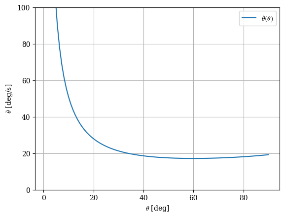
Substituting \(\dot s = 0.3\) m/s gives the angular velocity as a function of \(\theta\) alone.

Code
import sympy as sp
t = sp.symbols('t', real=True, positive=True)
theta_t = sp.Function('theta', real=True)(t)
s_t = sp.Function('s', real=True)(t)

eq = sp.Eq(s_t**2, s.subs(theta, theta_t)**2)
eq_dot = sp.Eq(sp.diff(eq.lhs, t), sp.diff(eq.rhs, t))
eq_dot | la

\[ {\def\arraystretch{1.0}2 s{\left(t \right)} \dfrac{d}{d t} s{\left(t \right)} = 4 \sin{\left(\theta{\left(t \right)} \right)} \dfrac{d}{d t} \theta{\left(t \right)}} \]

Code
import sympy as sp
omega_sym, s_dot_sym = sp.symbols(r'\omega \dot{s}', real=True, positive=True)
eq_dot = eq_dot.subs({
    sp.diff(theta_t, t): omega_sym,
    sp.diff(s_t, t): s_dot_sym,
    theta_t: theta,
    s_t: s,
})

omega = sp.simplify(sp.solve(eq_dot, omega_sym)[0])
omega = omega.subs(s_dot_sym, 0.3)

ltx(r"\dot\theta(\theta) =", omega, r"\text{ rad/s}")

\[ \dot\theta(\theta) =\dfrac{0.15 \sqrt{5 - 4 \cos{\left(\theta \right)}}}{\sin{\left(\theta \right)}}\text{ rad/s} \]

Plotting this over the opening range:

Code
import sympy as sp
theta_deg = sp.symbols('theta_deg')
fig, ax = plt.subplots()
fplot(omega.subs(theta, sp.rad(theta_deg))*180/sp.pi, (theta_deg, 1, 90), ax=ax, label=r'$\dot\theta(\theta)$')
ax.set(xlabel=r'$\theta$ [deg]', ylabel=r'$\dot\theta$ [deg/s]')
ax.set_ylim(0, 100)
ax.legend(); ax.grid(True)
plt.show()

Near \(\theta = 0\) the angular velocity diverges: the piston pulls almost along the arm \(OB\), so a small extension produces a large rotation. As \(\theta\) grows the curve flattens and appears to level off, but a closer look reveals a minimum around \(60^\circ\).

Code
import sympy as sp
theta_opt = sp.solve(sp.diff(omega, theta), theta)
theta_opt = [x for x in theta_opt if x.is_real and 0 < x < sp.pi/2][0]
omega_min = sp.simplify(omega.subs(theta, theta_opt))

ltx(r"\theta_{\min} =", theta_opt, r"=",
    sp.deg(theta_opt), r"^\circ,\qquad \dot\theta_{\min} =", omega_min, r"\text{ rad/s}")

\[ \theta_{\min} =1.0471975511966=\dfrac{188.495559215388}{\pi}^\circ,\qquad \dot\theta_{\min} =0.3\text{ rad/s} \]

The minimum is exactly \(60^\circ\) with \(\dot\theta_{\min} = 0.3\) rad/s.

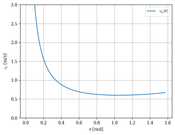
Peripheral speed at the bottom of the window

The bottom edge of the window is at a distance \(r = 2\) m from the hinge \(O\) (1 m to \(B\), then 1 m along the window). For pure rotation about \(O\) the speed of a point at radius \(r\) is

\[ v_p = r \dot\theta \]

Code
r = 2
v_p = r * omega
ltx(r"v_p(\theta) =", v_p, r"\text{ m/s}")

\[ v_p(\theta) =\dfrac{0.3 \sqrt{5 - 4 \cos{\left(\theta \right)}}}{\sin{\left(\theta \right)}}\text{ m/s} \]

Code
import sympy as sp
fig, ax = plt.subplots()
fplot(v_p, (theta, sp.pi/180, sp.pi/2), ax=ax, label=r'$v_p(\theta)$')
ax.set(xlabel=r'$\theta$ [rad]', ylabel=r'$v_p$ [m/s]')
ax.set_ylim(0, 3)
ax.legend(); ax.grid(True)
plt.show()

Angular acceleration

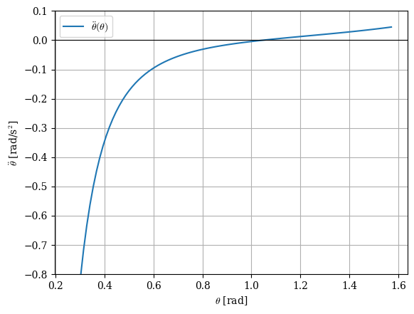
Differentiating \(\dot\theta(\theta)\) once more with respect to time and using the chain rule \(\ddot\theta = \dfrac{d\dot\theta}{d\theta}\,\dfrac{d\theta}{d t}\) gives the angular acceleration as a function of \(\theta\).

Code
import sympy as sp
alpha = sp.simplify(sp.diff(omega, theta) * omega)
ltx(r"\ddot\theta(\theta) =", alpha, r"\text{ rad/s}^2")

\[ \ddot\theta(\theta) =\dfrac{- 0.045 \sin^{2}{\left(\theta \right)} - 0.1125 \cos{\left(\theta \right)} + 0.09}{\sin^{3}{\left(\theta \right)}}\text{ rad/s}^2 \]

Code
import sympy as sp
fig, ax = plt.subplots()
fplot(alpha, (theta, sp.pi/12, sp.pi/2), ax=ax, label=r'$\ddot\theta(\theta)$')
ax.axhline(0, color='k', linewidth=0.8)
ax.set(xlabel=r'$\theta$ [rad]', ylabel=r'$\ddot\theta$ [rad/s$^2$]')
ax.set_ylim(-0.8, 0.1)
ax.legend(); ax.grid(True)
plt.show()

The angular acceleration is negative below \(60^\circ\) (the window is decelerating) and positive above (it is speeding up again), crossing zero exactly at the minimum of \(\dot\theta\). The stroke travels at constant rate, but the geometric mapping from stroke to angle is nonlinear, which is why a constant \(\dot s\) produces a non-constant \(\dot\theta\).

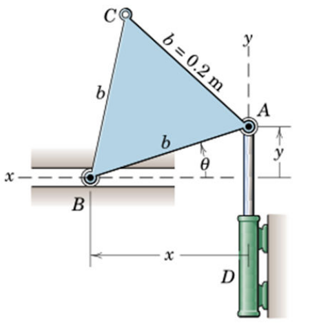
Example - Sliding triangular linkage

A rigid triangular plate \(CBA\) with sides \(b = 0.2\) m. Vertex \(B\) slides on a horizontal track, vertex \(A\) on a vertical track. Vertex \(A\) moves down at \(v_A = 0.3\) m/s.

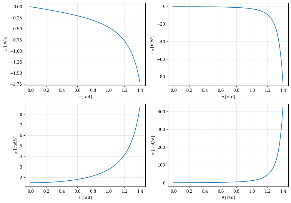
Find \(v_B(\theta)\), \(a_B(\theta)\), \(\omega(\theta)\), and \(\alpha(\theta)\) for \(\theta \in [0, 80^\circ]\), where \(\theta\) is the angle of bar \(BA\) above the horizontal.

Solution

With the origin at the corner where the tracks meet, \(A_y = b\sin\theta\) and \(B_x = b\cos\theta\). Differentiating \(A_y^2 + B_x^2 = b^2\) in time and using \(\dot A_y = v_A\) propagates the kinematics.

Differentiate \(A_y(t) = b\sin\theta(t)\) in time using the chain rule, then apply \(\dot A_y = v_A\) to solve for the angular velocity \(\dot\theta = \omega\):

Code
t = sp.symbols('t', real=True)
b, v_A_sym = sp.symbols('b v_A', positive=True)
theta = sp.Function(r'\theta')

A_y = b * sp.sin(theta(t))
dA_y_dt = sp.diff(A_y, t)
theta_dot = sp.solve(sp.Eq(dA_y_dt, v_A_sym), sp.diff(theta(t), t))[0]

ltx(
    r"A_y &=", A_y, r"\\",
    r"\dot A_y &=", dA_y_dt, r"\\",
    r"\dot A_y = v_A \;\implies\; \omega = \dot\theta &=", theta_dot, r"\text{ rad/s}",
    aligned=True,
)

\[ \begin{aligned}A_y &=b \sin{\left(\theta{\left(t \right)} \right)}\\\dot A_y &=b \cos{\left(\theta{\left(t \right)} \right)} \dfrac{d}{d t} \theta{\left(t \right)}\\\dot A_y = v_A \;\implies\; \omega = \dot\theta &=\dfrac{v_{A}}{b \cos{\left(\theta{\left(t \right)} \right)}}\text{ rad/s}\end{aligned} \]

Code
B_x = b * sp.cos(theta(t))
v_B_t = sp.diff(B_x, t).subs(sp.diff(theta(t), t), theta_dot)
a_B_t = sp.diff(v_B_t, t).subs(sp.diff(theta(t), t), theta_dot)

ltx(
    r"B_x &=", B_x, r"\\",
    r"\dot B_x &=", sp.diff(B_x, t), r"\\",
    r"v_B(t) &=", v_B_t, r"\text{ m/s} \\",
    r"a_B(t) &=", a_B_t, r"\text{ m/s}^2",
    aligned=True,
)

\[ \begin{aligned}B_x &=b \cos{\left(\theta{\left(t \right)} \right)}\\\dot B_x &=- b \sin{\left(\theta{\left(t \right)} \right)} \dfrac{d}{d t} \theta{\left(t \right)}\\v_B(t) &=- \dfrac{v_{A} \sin{\left(\theta{\left(t \right)} \right)}}{\cos{\left(\theta{\left(t \right)} \right)}}\text{ m/s} \\a_B(t) &=- \dfrac{v_{A}^{2} \sin^{2}{\left(\theta{\left(t \right)} \right)}}{b \cos^{3}{\left(\theta{\left(t \right)} \right)}} - \dfrac{v_{A}^{2}}{b \cos{\left(\theta{\left(t \right)} \right)}}\text{ m/s}^2\end{aligned} \]

Code
omega_t = theta_dot
alpha_t = sp.diff(omega_t, t).subs(sp.diff(theta(t), t), theta_dot)
ltx(r"\omega(t) &=", omega_t, r"\text{ rad/s},\\ ",
    r"\alpha(t) &=", alpha_t, r"\text{ rad/s}^2",
    aligned=True)

\[ \begin{aligned}\omega(t) &=\dfrac{v_{A}}{b \cos{\left(\theta{\left(t \right)} \right)}}\text{ rad/s},\\ \alpha(t) &=\dfrac{v_{A}^{2} \sin{\left(\theta{\left(t \right)} \right)}}{b^{2} \cos^{3}{\left(\theta{\left(t \right)} \right)}}\text{ rad/s}^2\end{aligned} \]

Code
theta_sym = sp.symbols(r'\theta', real=True)
# Substitute theta(t) with a symbolic variable 
# to express v_B, a_B, omega, alpha as functions of theta
as_theta = lambda e: sp.simplify(e.subs(theta(t), theta_sym))

v_B   = as_theta(v_B_t)
a_B   = as_theta(a_B_t)
omega = as_theta(omega_t)
alpha = as_theta(alpha_t)

ltx(
    r"v_B(\theta) &=", v_B,   r"\text{ m/s} \\",
    r"a_B(\theta) &=", a_B,   r"\text{ m/s}^2 \\",
    r"\omega(\theta) &=", omega, r"\text{ rad/s} \\",
    r"\alpha(\theta) &=", alpha, r"\text{ rad/s}^2",
    aligned=True,
)

\[ \begin{aligned}v_B(\theta) &=- v_{A} \tan{\left(\theta \right)}\text{ m/s} \\a_B(\theta) &=- \dfrac{v_{A}^{2}}{b \cos^{3}{\left(\theta \right)}}\text{ m/s}^2 \\\omega(\theta) &=\dfrac{v_{A}}{b \cos{\left(\theta \right)}}\text{ rad/s} \\\alpha(\theta) &=\dfrac{v_{A}^{2} \sin{\left(\theta \right)}}{b^{2} \cos^{3}{\left(\theta \right)}}\text{ rad/s}^2\end{aligned} \]

Code
nums = {v_A_sym: 0.3, b: 0.2}
specs = [
    (v_B.subs(nums),   r'$v_B$ [m/s]'),
    (a_B.subs(nums),   r'$a_B$ [m/s$^2$]'),
    (omega.subs(nums), r'$\omega$ [rad/s]'),
    (alpha.subs(nums), r'$\alpha$ [rad/s$^2$]'),
]
fig, axes = plt.subplots(2, 2, figsize=(10, 7))
for (expr, ylabel), ax in zip(specs, axes.flat):
    fplot(expr, (theta_sym, 0, 80*sp.pi/180), ax=ax)
    ax.set_xlabel(r'$\theta$ [rad]')
    ax.set_ylabel(ylabel)
    ax.grid(True, alpha=0.3)
plt.tight_layout()
plt.show()

Rotation

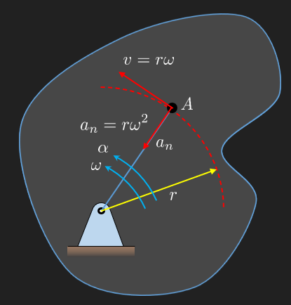
A rigid body rotating about a fixed axis is the simplest case of plane motion: every point traces a circle, and a single scalar \(\omega(t)\) together with the radius fixes the velocity and acceleration of every point. This section promotes the scalar relations \(v = r\omega\) and \(a_n = r\omega^2\) to vector form using cross products, which extends cleanly to the moving-pivot case in the next section.

General plane motion of a rigid body

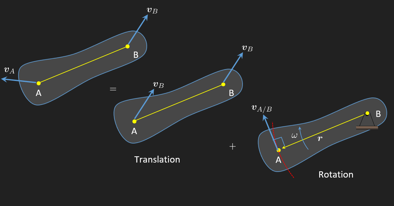
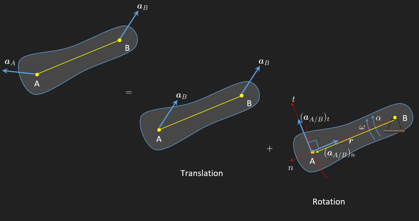
The same motion decomposed into a translation and a rotation

A body rotating about a fixed point. The fixed point may be on or outside the body.

We recall from Section 6.3.12 that for a particle tracing a circle of radius \(r\)

\[ \begin{aligned} & v = r \omega \\ & a_n = r\omega^2 = \dfrac{v^2}{R} \\ & a_t = r \alpha = \dot v \end{aligned} \]

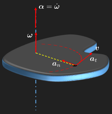
Rotation about the \(z\)-axis in 3D. The scalar relations of the 2D case carry over once we express \(\bm\omega\), \(\bm\alpha\) and the position as vectors and replace products by cross products.

In three dimensions we promote \(\omega\) to a vector \(\bm\omega = \omega\,\bm e_z\) aligned with the rotation axis. Its direction follows from the right-hand rule: a body spinning at 5 rad/s about \(\bm e_z\) rotates counter-clockwise when viewed from the \(+z\) side.

With this promotion the kinematic relations take a coordinate-free vector form,

\[ \begin{aligned} & \bm v = \bm\omega \times \bm r \\ & \bm a_n = \bm\omega \times (\bm\omega \times \bm r) \\ & \bm a_t = \bm\alpha \times \bm r \\ & \bm a = \bm a_n + \bm a_t \end{aligned} \]

The right-hand rule fixes the direction of each cross product. With \(\bm\omega\) along \(+\bm e_z\), aligning the thumb with \(\bm\omega\) and the index finger with \(\bm r\) sends the middle finger along \(\bm v\). Geometrically, \(\bm\omega \times \bm r\) rotates \(\bm r\) by \(90^\circ\) in the plane perpendicular to \(\bm\omega\), giving a velocity tangent to the circular path. Applying the rule again, \(\bm a_n = \bm\omega \times \bm v\) rotates \(\bm v\) by another \(90^\circ\) and thus points from the particle toward the rotation axis, which is the centripetal direction.

The vector formulas become concrete once we write out the components. Take \(\bm\omega = \omega\,\bm e_z\) for a body spinning about the \(z\)-axis and place a point at \(\bm r_A = r \bm e_x\), so

\[ \bm\omega = \begin{bmatrix} 0 \\ 0 \\ \omega \end{bmatrix}, \qquad \bm r_A = r \begin{bmatrix} 1 \\ 0 \\ 0 \end{bmatrix}. \]

The velocity follows directly from the cross product,

\[ \bm v_A = \bm\omega \times \bm r_A = \omega \begin{bmatrix} 0 \\ 0 \\ 1 \end{bmatrix} \times r \begin{bmatrix} 1 \\ 0 \\ 0 \end{bmatrix} = \begin{bmatrix} 0\cdot 0 - \omega\cdot 0 \\ \omega\cdot r - 0\cdot 0 \\ 0\cdot 0 - 0\cdot r \end{bmatrix} = r \omega\begin{bmatrix} 0 \\ 1 \\ 0 \end{bmatrix} = r \omega\,\bm e_y. \]

The result has magnitude \(r \omega\) and points along \(+\bm e_y\), perpendicular to both \(\bm\omega\) and \(\bm r_A\) as the right-hand rule predicts. This is the tangent direction at the particle’s circular path, and the scalar relation \(v = r\omega\) of the 2D case is recovered.

Applying the cross product once more gives the normal (centripetal) acceleration,

\[ \bm a_n = \bm\omega \times \bm v_A = \omega \begin{bmatrix} 0 \\ 0 \\ 1 \end{bmatrix} \times r \omega \begin{bmatrix} 0 \\ 1 \\ 0 \end{bmatrix} = \begin{bmatrix} 0\cdot 0 - \omega \cdot r \omega \\ \omega\cdot 0 - 0\cdot 0 \\ 0\cdot r \omega - 0\cdot 0 \end{bmatrix} = r\omega^2 \begin{bmatrix} - 1 \\ 0 \\ 0 \end{bmatrix} = -r\omega^2\,\bm e_x. \]

The acceleration points back along \(-\bm e_x\), from the particle toward the rotation axis, with magnitude \(r \omega^2\). This matches \(a_n = r\omega^2\) from the scalar case. Each cross product with \(\bm\omega\) rotates the previous vector by \(90^\circ\) in the plane perpendicular to the rotation axis: \(\bm r\) becomes the tangent direction of \(\bm v\), and \(\bm v\) becomes the inward radial direction of \(\bm a_n\).

Rotation Example - Gearing

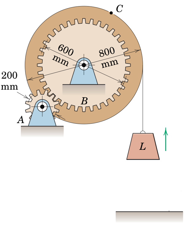
Pinion \(A\) (radius \(r_A = 200\) mm) drives gear \(B\) (pitch radius \(r_B = 600\) mm), which is fixed to a hoisting drum of radius \(r_D = 800\) mm. A cable wound on the drum lifts the load \(L\). Point \(C\) sits on the drum rim.

Pinion \(A\) drives gear \(B\), which is rigidly attached to a hoisting drum of radius \(r_D = 800\) mm. A cable wound on the drum lifts the load \(L\). At the instant shown the pinion rotates at \(\omega_A = 200\) rpm and is accelerating at \(\alpha_A = 10\) rad/s\(^2\). We want

  • the velocity \(v_L\) and acceleration \(a_L\) of the load, and
  • the acceleration of point \(C\) on the drum rim.

Solution

The hoist forms a single kinematic chain carrying the pinion’s motion outward to the load. The pinion-gear mesh imposes a no-slip rolling contact (see below) that fixes the drum’s angular velocity. The cable leaves the drum tangentially, so the load moves with the drum’s rim speed at the cable point, \(v_L = r_D\omega_B\). Differentiating both constraints once in time propagates accelerations along the same chain.

ImportantNo-slip at a rolling contact

Where two rotating bodies meet without slipping, whether gear teeth, friction wheels, a chain on a sprocket, or a wheel on the ground, the surface velocities at the contact point are equal. For two cylinders of radii \(r_1\) and \(r_2\) rotating at \(\omega_1\) and \(\omega_2\), the no-slip condition gives

\[ r_1\,\omega_1 = r_2\,\omega_2. \]

This single equation is what links one rotating element to the next in a kinematic chain, and the same form appears in every problem involving gears, belts, or rolling motion.

Converting the pinion speed to SI units, \(\omega_A = 200 \cdot 2\pi/60\) rad/s. Solving the two constraints for the drum and the load gives

\[ \omega_B = \frac{r_A}{r_B}\,\omega_A, \qquad v_L = r_D\,\omega_B \]

and the same relations with \(\alpha\) in place of \(\omega\) and \(a_L\) in place of \(v_L\) for the accelerations.

Code
import sympy as sp
from mechanicskit import ltx

r_A = 0.2
r_B = 0.6
r_D = 0.8
omega_A = 200 * 2 * sp.pi / 60
alpha_A = 10

omega_B = omega_A * r_A / r_B
alpha_B = alpha_A * r_A / r_B
v_L = r_D * omega_B
a_L = r_D * alpha_B

ltx(
    r"\omega_B &=", omega_B, r"\text{ rad/s} \\",
    r"\alpha_B &=", alpha_B, r"\text{ rad/s}^2 \\",
    r"v_L &=", v_L, r"\text{ m/s} \\",
    r"a_L &=", a_L, r"\text{ m/s}^2",
    aligned=True, precision=4,
)

\[ \begin{aligned}\omega_B &=6.981\text{ rad/s} \\\alpha_B &=3.3333\text{ rad/s}^2 \\v_L &=5.585\text{ m/s} \\a_L &=2.6667\text{ m/s}^2\end{aligned} \]

Point \(C\) rides on the drum rim at radius \(r_D\), so its acceleration splits into a tangential component along the rim and a normal component pointing toward the drum centre,

\[ a_t^C = r_D\,\alpha_B, \qquad a_n^C = r_D\,\omega_B^2 \]

The two are perpendicular and the magnitude is the Pythagorean sum.

Code
a_n_C = omega_B**2 * r_D
a_t_C = alpha_B * r_D
a_C = sp.sqrt(a_n_C**2 + a_t_C**2)

ltx(
    r"a_n^C &=", a_n_C, r"\text{ m/s}^2 \\",
    r"a_t^C &=", a_t_C, r"\text{ m/s}^2 \\",
    r"|\bm a_C| &=", a_C, r"\text{ m/s}^2",
    aligned=True, precision=4,
)

\[ \begin{aligned}a_n^C &=38.99\text{ m/s}^2 \\a_t^C &=2.6667\text{ m/s}^2 \\|\bm a_C| &=39.08\text{ m/s}^2\end{aligned} \]

Rotation Example - Rotating bar

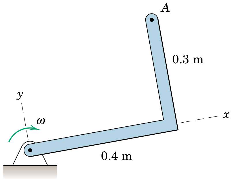
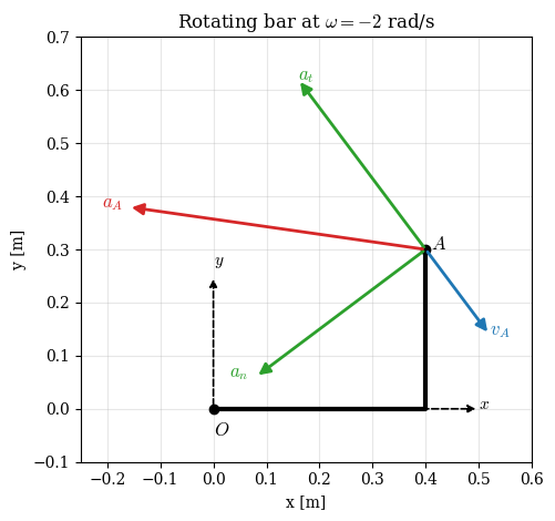
A right-angle bar is rotating around a fixed axis.

The right-angle bar rotates clockwise with an angular velocity decreasing at the rate of \(4~\text{rad/s}^2\). Write the vector expressions for the velocity and acceleration of point \(A\) when \(\omega = 2~\text{rad/s}\).

Solution

We place the origin at the bar’s pivot, with \(\bm e_x\) along the horizontal segment, \(\bm e_y\) along the vertical segment, and \(\bm e_z\) out of the figure plane along the rotation axis. Point \(A\) sits at

\[ \bm r_{OA} = 0.4\,\bm e_x + 0.3\,\bm e_y \text{ m}. \]

The bar rotates clockwise as viewed from the \(+\bm e_z\) side (the reader’s viewpoint), so the angular velocity vector points along \(-\bm e_z\),

\[ \bm\omega = -2\,\bm e_z \text{ rad/s}. \]

The magnitude of \(\bm\omega\) is decreasing at \(\alpha=\) 4 rad/s\(^2\), which means the angular acceleration vector opposes \(\bm\omega\) and therefore points along \(+\bm e_z\),

\[ \bm\alpha = 4\,\bm e_z \text{ rad/s}^2. \]

Both \(\bm\omega\) and \(\bm\alpha\) are perpendicular to the plane of the bar, so the full position vector \(\bm r_{OA}\) enters the cross products. The perpendicular distance from \(A\) to the rotation axis is \(r_\perp = |\bm r_{OA}| = \sqrt{0.4^2 + 0.3^2} = 0.5\) m. The velocity and the two acceleration components follow from \(\bm v_A = \bm\omega \times \bm r_{OA}\), \(\bm a_n = \bm\omega \times \bm v_A\), and \(\bm a_t = \bm\alpha \times \bm r_{OA}\).

Code
rr_OA = sp.Matrix([0.4, 0.3, 0])
omega = sp.Matrix([0, 0, -2])
alpha = sp.Matrix([0, 0,  4])

vv_A = omega.cross(rr_OA)
aa_n = omega.cross(vv_A)
aa_t = alpha.cross(rr_OA)
aa_A = aa_n + aa_t

ltx(
    r"\bm v_A &=", vv_A, r"\text{ m/s} \\",
    r"\bm a_n &=", aa_n, r"\text{ m/s}^2 \\",
    r"\bm a_t &=", aa_t, r"\text{ m/s}^2 \\",
    r"\bm a_A &=", aa_A, r"\text{ m/s}^2",
    aligned=True,
)

\[ \begin{aligned}\bm v_A &=\left[\begin{matrix}0.6\\-0.8\\0\end{matrix}\right]\text{ m/s} \\\bm a_n &=\left[\begin{matrix}-1.6\\-1.2\\0\end{matrix}\right]\text{ m/s}^2 \\\bm a_t &=\left[\begin{matrix}-1.2\\1.6\\0\end{matrix}\right]\text{ m/s}^2 \\\bm a_A &=\left[\begin{matrix}-2.8\\0.4\\0\end{matrix}\right]\text{ m/s}^2\end{aligned} \]

The velocity \(\bm v_A = 0.6\,\bm e_x - 0.8\,\bm e_y\) m/s is tangent to the circular path of \(A\) in the figure plane, with magnitude \(r_\perp \omega = 0.5 \cdot 2 = 1\) m/s. The normal acceleration \(\bm a_n = -1.6\,\bm e_x - 1.2\,\bm e_y\) m/s\(^2\) points from \(A\) back toward the origin (where the rotation axis pierces the plane), with magnitude \(r_\perp\,\omega^2 = 2\) m/s\(^2\). The tangential acceleration \(\bm a_t = -1.2\,\bm e_x + 1.6\,\bm e_y\) m/s\(^2\) is antiparallel to \(\bm v_A\), as expected for a slowing rotation, and has magnitude \(r_\perp\,|\bm\alpha| = 2\) m/s\(^2\). Adding the two perpendicular components,

\[ \bm a_A = -2.8\,\bm e_x + 0.4\,\bm e_y \text{ m/s}^2, \qquad |\bm a_A| = 2\sqrt{2} \approx 2.83 \text{ m/s}^2. \]

A picture of the geometry and the kinematic vectors at the instant \(\omega = 2\) rad/s, with the bar in the figure plane and rotation axis \(\bm e_z\) pointing toward the reader.

Code
from mechanicskit import arrow

A = sp.Matrix([0.4, 0.3, 0])

fig, ax = plt.subplots()

# Bar
ax.plot([0, 0.4, 0.4], [0, 0, 0.3], color='k', lw=3, solid_capstyle='round')

# Origin and point A markers
ax.plot(0, 0, 'ko', ms=6)
ax.plot(0.4, 0.3, 'ko', ms=6)
ax.text(0, -0.05, '$O$', fontsize=12)
ax.text(0.41, 0.3, '$A$', fontsize=12)

# Local x and y axes at the origin
arrow([0, 0], [0.5, 0], ax=ax, color='k', linestyle='--', linewidth=1.2, head_scale =10)
arrow([0, 0], [0, 0.25], ax=ax, color='k', linestyle='--', linewidth=1.2, head_scale =10)
ax.text(0.5, 0, '$x$', color='k', fontsize=11)
ax.text(0, 0.27, '$y$', color='k', fontsize=11)

# Velocity (blue), acceleration components (green), resultant (red)
scale = 0.2
arrow(A, vv_A, ax=ax, color='tab:blue', scale=scale)
arrow(A, aa_n, ax=ax, color='tab:green', scale=scale)
arrow(A, aa_t, ax=ax, color='tab:green', scale=scale)
arrow(A, aa_A, ax=ax, color='tab:red', scale=scale)

# Tip labels
ax.text(0.4 + float(vv_A[0])*scale, 0.3 + float(vv_A[1])*scale, r'$v_A$', color='tab:blue',  fontsize=12)
ax.text(0.4 + float(aa_n[0])*scale-0.05, 0.3 + float(aa_n[1])*scale, r'$a_n$', color='tab:green', fontsize=12)
ax.text(0.4 + float(aa_t[0])*scale, 0.3 + float(aa_t[1])*scale, r'$a_t$', color='tab:green', fontsize=12)
ax.text(0.4 + float(aa_A[0])*scale-0.05, 0.3 + float(aa_A[1])*scale, r'$a_A$', color='tab:red',   fontsize=12)

ax.set_aspect('equal')
ax.grid(True, alpha=0.3)
ax.set_xlabel('x [m]'); ax.set_ylabel('y [m]')
ax.set_title(r'Rotating bar at $\omega = -2$ rad/s')
ax.set_xlim(-0.25, 0.6)
ax.set_ylim(-0.1, 0.7)
plt.tight_layout()
plt.show()

Relative Motion

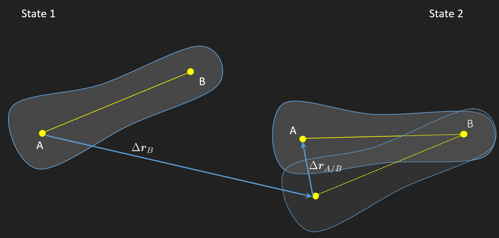
The rotation formulas above assume a fixed pivot. When the body translates as well as rotates, we describe each point relative to a chosen reference point that itself moves. The motion of any other point splits into two pieces: the motion of the reference and a rotation about it. The animations below illustrate this decomposition.

The motion is expressed as the sum of a parallel translation of point B, \(\bm r_B\), and the relative translation \(\bm r_{A/B}\) (“A seen from B”)

\[ \boxed{ \Delta \bm r_A = \Delta \bm r_B + \Delta \bm r_{A/B} } \]

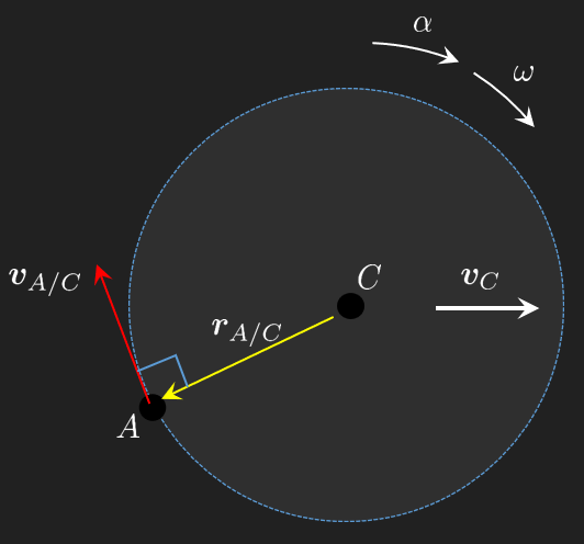
Differentiating the position relation in time gives the velocity decomposition. The body-fixed offset \(\bm r\) has constant length, so its time derivative is purely rotational, \(\dot{\bm r} = \bm\omega \times \bm r\), perpendicular to \(\bm r\) with magnitude \(\omega r\).

Relative velocity

\[ \boxed{ \begin{array}{rlr} \bm v_A & = \bm v_B + \bm v_{A/B} \qquad v_{A/B} = \omega r \\ & = \bm v_B + \bm\omega \times \bm r & \end{array} } \]

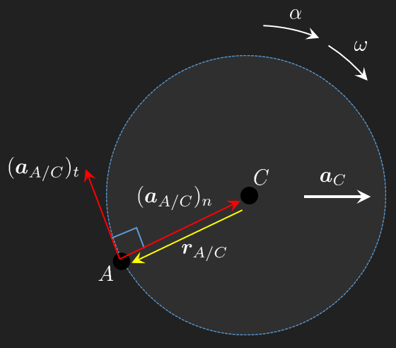
A second time derivative gives the acceleration. The relative term picks up two pieces, mirroring the centripetal-tangential split for a particle on a circular path:

Relative acceleration

\[ \boxed{ \begin{aligned} \boldsymbol{a}_A & =\boldsymbol{a}_B+\boldsymbol{a}_{A / B} \\ & =\boldsymbol{a}_B+\left(\boldsymbol{a}_{A / B}\right)_n+\left(\boldsymbol{a}_{A / B}\right)_t \end{aligned} } \]

The two components have the same form as for a particle on a circle of radius \(r\) centred on \(B\), with \(\bm r\) playing the role of the radius vector:

\[ \boxed{ \begin{array}{ll} \left(\bm{a}_{A / B}\right)_n=\bm{\omega} \times(\bm{\omega} \times \bm{r}) & \quad \left(\bm{a}_{A / B}\right)_t=\bm{\alpha} \times \bm{r} \\[1.0em] \left(a_{A / B}\right)_n=v_{A / B}^2 / r=r \omega^2 & \quad \left(a_{A / B}\right)_t=\dot{v}_{A / B}=r \alpha \end{array} } \]

Example - Rolling wheel - Relative motion

We revisit the rolling wheel of Section 6.4.1 using the centre \(C\) as reference. \(C\) travels in a straight line at \(r\omega\), so its velocity and acceleration are known. The rim point \(A\) swings about \(C\) on a circle of radius \(r\), and the relative formulas reduce to a single cross product per derivative.

\[ \boxed{\Delta \bm r_A = \Delta \bm r_B + \Delta \bm r_{A/B}} \Rightarrow \bm r_A = \bm r_C + \bm r_{A/C} \]

\[ \bm{r}_{A}=\overset{\bm{r}_{C}}{\overbrace{\begin{bmatrix}r\theta\\ r\\ 0 \end{bmatrix}}}+\overset{\bm{r}_{A/C}}{\overbrace{r\begin{bmatrix}-\sin\theta\\ -\cos\theta\\ 0 \end{bmatrix}}} \]

\[ \boldsymbol{r}_A=\left[\begin{array}{c} r \theta-r \sin \theta \\ r-r \cos \theta \\ 0 \end{array}\right] \]

Relative velocity

\[ \boxed{ \begin{aligned} & \boldsymbol{v}_A=\boldsymbol{v}_B+\boldsymbol{v}_{A / B} \\ & v_{A / B}=\omega r \\ & \boldsymbol{v}_{A / B}=\boldsymbol{\omega} \times \boldsymbol{r} \end{aligned} } \]

Relative velocity

\[ \begin{aligned} & \boldsymbol{v}_A=\boldsymbol{v}_C+\boldsymbol{v}_{A / C} \\ & \boldsymbol{v}_{A / C}=\boldsymbol{\omega} \times \boldsymbol{r}_{A / C} \end{aligned} \]

\[ \underbrace{\left[\begin{array}{c} r \omega \\ 0 \\ 0 \end{array}\right]}_{v_C}+\underbrace{\left[\begin{array}{c} 0 \\ 0 \\ -\omega \end{array}\right]}_\omega \times \underbrace{r\left[\begin{array}{c} -\sin \theta \\ -\cos \theta \\ 0 \end{array}\right]}_{r_{A / C}}=\underbrace{\left[\begin{array}{c} r \omega(1-\cos \theta) \\ r \omega \sin \theta \\ 0 \end{array}\right]}_{v_A} \]

At the contact point (\(\theta = 0\)), \(\bm v_A = \bm 0\): the contact is instantaneously at rest, which is the statement of rolling without slipping. At the top of the wheel (\(\theta = \pi\)), \(\bm v_A = 2 r\omega \bm e_x\), twice the centre speed.

Relative acceleration

Relative acceleration

\[ \boxed{ \begin{aligned} & \bm a_A = \bm a_B + \bm a_{A/B} \\ & \quad = \bm a_B + \left(\bm a_{A/B}\right)_n + \left(\bm a_{A/B}\right)_t \\ & \quad \left(\bm a_{A/B}\right)_n = \bm\omega \times (\bm\omega \times \bm r) \quad \left(\bm a_{A/B}\right)_t = \bm\alpha \times \bm r \end{aligned} } \]

\[ \begin{aligned} & \boldsymbol{a}_A=\boldsymbol{a}_C+\left(\boldsymbol{a}_{A / C}\right)_n+\left(\boldsymbol{a}_{A / C}\right)_t \\ & \left(\boldsymbol{a}_{A / C}\right)_n=\boldsymbol{\omega} \times\left(\boldsymbol{\omega} \times \boldsymbol{r}_{A / C}\right) \\ & \left(\boldsymbol{a}_{A / C}\right)_t=\boldsymbol{\alpha} \times \boldsymbol{r}_{A / C} \end{aligned} \]

\[ \left(\boldsymbol{a}_{A / C}\right)_n=\underbrace{\left[\begin{array}{c} 0 \\ 0 \\ -\omega \end{array}\right]}_\omega \times \underbrace{\left[\begin{array}{c} 0 \\ 0 \\ -\omega \end{array}\right]}_\omega \times \underbrace{r\left[\begin{array}{c} -\sin \theta \\ -\cos \theta \\ 0 \end{array}\right]}_{r_{A / C}}=r \omega^2\left[\begin{array}{c} \sin \theta \\ \cos \theta \\ 0 \end{array}\right] \]

\[ \left(\boldsymbol{a}_{A / C}\right)_t=\underbrace{\left[\begin{array}{c} 0 \\ 0 \\ -\alpha \end{array}\right]}_\alpha \times \underbrace{r\left[\begin{array}{c} -\sin \theta \\ -\cos \theta \\ 0 \end{array}\right]}_{r_{A / C}}=r \alpha\left[\begin{array}{c} -\cos \theta \\ \sin \theta \\ 0 \end{array}\right] \]

\[ \underbrace{\left[\begin{array}{c} r \alpha \\ 0 \\ 0 \end{array}\right]}_{\boldsymbol{a}_C}+\underbrace{r \omega^2\left[\begin{array}{c} \sin \theta \\ \cos \theta \\ 0 \end{array}\right]}_{\left(\boldsymbol{a}_{A / C}\right)_n}+\underbrace{r \alpha\left[\begin{array}{c} -\cos \theta \\ \sin \theta \\ 0 \end{array}\right]}_{\left(\boldsymbol{a}_{A / C}\right)_t}=\left[\begin{array}{c} \alpha r (1-\cos \theta)+\omega^2 r \sin (\theta) \\ \omega^2 r \cos (\theta)+\alpha r \sin (\theta) \\ 0 \end{array}\right] \]

This is exactly \(\ddot P\) from the absolute-motion derivation, recovered without parameterising the cycloid by time. At the contact point (\(\theta = 0\)), \(\bm a_A = (0, r\omega^2, 0)^\mathsf T\): purely centripetal toward the centre, even though the contact velocity is zero. The contact point of a rolling wheel is at rest instantaneously, not over any finite interval.

Example - Hydraulic crank linkage

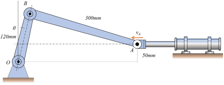
A hydraulic cylinder pushes the slider \(A\) horizontally to the left at constant speed \(v_A = 2\) m/s. The slider connects through a rigid link of length \(L_{BA} = 300\) mm to the end of a crank \(OB\) of length \(L_{OB} = 120\) mm pinned at the fixed pivot \(O\). The slider track sits \(h = 50\) mm above the pivot. We want the angular velocities \(\omega_O\) of the crank and \(\omega_{BA}\) of the connecting rod when the crank makes an angle \(\theta = 20^\circ\) with the upward vertical.

Hydraulic cylinder

Solution

Place the origin at the pivot \(O\) with \(\bm e_x\) horizontal and \(\bm e_y\) pointing up, and let \(\theta\) be the angle of \(OB\) measured from the upward vertical. The crank end is at

\[ \bm r_{OB}(\theta) = L_{OB}\begin{bmatrix}\sin\theta\\\cos\theta\\0\end{bmatrix}. \]

The slider rides on the horizontal track \(y = h\), to the right of \(B\). The fixed length \(|\bm r_{AB}| = L_{BA}\) pins down its \(x\)-coordinate, and the connecting-rod vector reads

\[ \bm r_{AB}(\theta) = \begin{bmatrix}-\sqrt{L_{BA}^2 - (L_{OB}\cos\theta - h)^2}\\L_{OB}\cos\theta - h\\0\end{bmatrix}. \]

Code
theta = sp.symbols('theta', real=True, positive=True)
omega_O, omega_BA = sp.symbols(r'\omega_O \omega_{BA}', real=True)

L_OB = sp.Rational(120, 1000)
L_BA = sp.Rational(300, 1000)
h    = sp.Rational(50, 1000)

rr_OB = L_OB * sp.Matrix([sp.sin(theta), sp.cos(theta), 0])
R_y = L_OB*sp.cos(theta) - h
R_x = -sp.sqrt(L_BA**2 - R_y**2)
rr_AB = sp.Matrix([R_x, R_y, 0])

ltx(r"\bm r_{OB} &=", rr_OB, r"\text{ m} \\",
    r"\bm r_{AB} &=", rr_AB, r"\text{ m}", aligned=True)

\[ \begin{aligned}\bm r_{OB} &=\left[\begin{matrix}\dfrac{3 \sin{\left(\theta \right)}}{25}\\\dfrac{3 \cos{\left(\theta \right)}}{25}\\0\end{matrix}\right]\text{ m} \\\bm r_{AB} &=\left[\begin{matrix}- \sqrt{\dfrac{9}{100} - \left(\dfrac{3 \cos{\left(\theta \right)}}{25} - \dfrac{1}{20}\right)^{2}}\\\dfrac{3 \cos{\left(\theta \right)}}{25} - \dfrac{1}{20}\\0\end{matrix}\right]\text{ m}\end{aligned} \]

The relative-velocity equation links the two angular velocities to the slider speed,

\[ \bm v_B = \bm v_A + \bm v_{B/A}, \qquad \bm\omega_O \times \bm r_{OB} = \bm v_A + \bm\omega_{BA} \times \bm r_{AB}, \]

with \(\bm v_A = -2\,\bm e_x\) m/s and both angular velocities along \(\bm e_z\). The \(z\)-component of the equation vanishes, so the \(x\) and \(y\) components form a \(2\times 2\) linear system for \(\omega_O\) and \(\omega_{BA}\).

Code
ww_O  = sp.Matrix([0, 0, omega_O])
ww_BA = sp.Matrix([0, 0, omega_BA])
vv_A  = sp.Matrix([-2, 0, 0])

eqs = [sp.Eq(l, r) for l, r in zip(ww_O.cross(rr_OB), vv_A + ww_BA.cross(rr_AB))]
sol = sp.solve(eqs, [omega_O, omega_BA])

theta_20 = 20 * sp.pi / 180
ltx(r"\omega_O &=", sol[omega_O].subs(theta, theta_20).evalf(5), r"\text{ rad/s} \\",
    r"\omega_{BA} &=", sol[omega_BA].subs(theta, theta_20).evalf(5), r"\text{ rad/s}",
    aligned=True)

\[ \begin{aligned}\omega_O &=16.455\text{ rad/s} \\\omega_{BA} &=-2.3021\text{ rad/s}\end{aligned} \]

The crank rotates counter-clockwise at about 16.5 rad/s while the connecting rod swings the opposite way at about 2.3 rad/s. The mechanism becomes singular as the connecting rod approaches the horizontal: a horizontal \(\bm r_{AB}\) has no \(y\)-component, so the \(y\)-equation can no longer balance the \(\sin\theta\) contribution from \(\bm\omega_O \times \bm r_{OB}\), and \(\omega_O\) blows up.

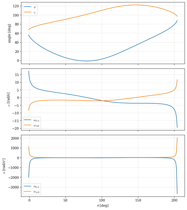
Example - Three-bar mechanism

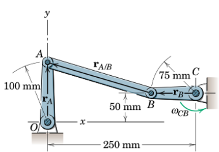
Three-bar linkage. The crank \(CB\) is the input, the crank \(OA\) is the output, and the connecting rod \(AB\) ties them together. Lengths are 100 mm, 182 mm, and 75 mm; the fixed pivots are at \(O\) and \(C = (250, 50)\) mm.

The crank \(CB\) rotates at constant \(\omega_{CB} = 5\) rad/s. We want the link positions, the angular velocities \(\omega_{OA}\), \(\omega_{AB}\), and the angular accelerations \(\alpha_{OA}\), \(\alpha_{AB}\) as functions of the input angle \(\theta\) that locates \(CB\).

Three-bar mechanisms differ from the slider-crank in one respect: the loop closure is implicit. There is no closed-form expression for \(A\) given \(\theta\), so we solve numerically.

Preliminary analysis

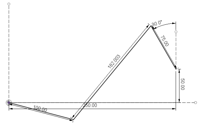
Sketching the configuration in CAD before writing equations is worth the time. The same set of link lengths admits two assemblies at most input angles, and the model has to land on the intended branch.

Alternative assembly at the same input angle \(\theta = 30^\circ\). Two configurations exist for most \(\theta\); warm-starting the nonlinear solver from the previous solution keeps the swept trajectory on a single branch.

Position analysis

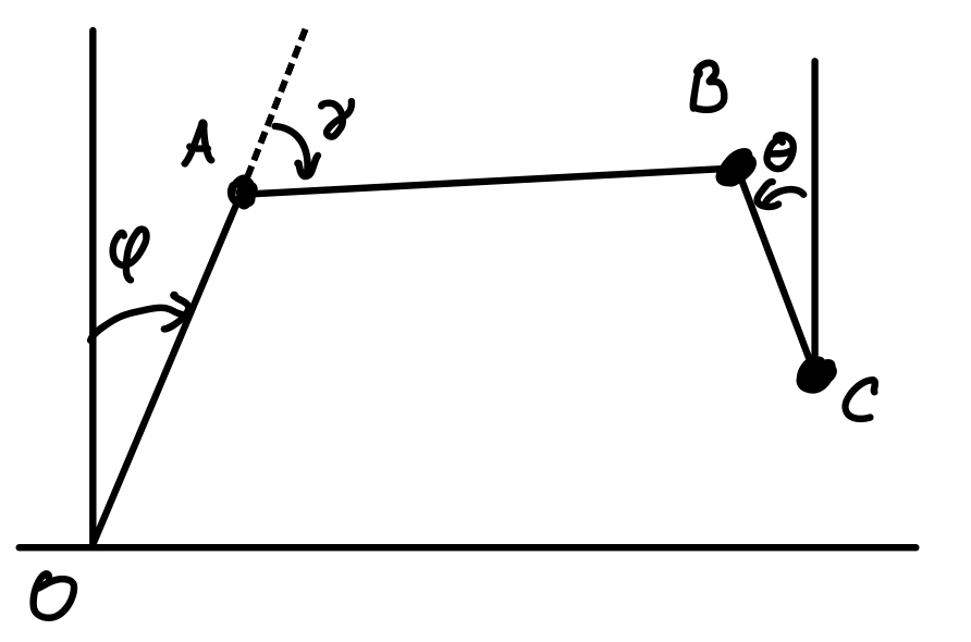
We close the kinematic loop \(O \to A \to B\) and equate it to \(O \to C \to B\). Let \(\varphi\) be the angle of \(OA\) from the upward vertical and \(\gamma\) the angle of \(AB\) from the upward vertical. Then

\[ \bm r_{OA}(\varphi) + \bm r_{AB}(\varphi, \gamma) = \bm r_{OC} + \bm r_{CB}(\theta). \]

For each \(\theta\) this is a \(2\times 2\) nonlinear system in \((\varphi, \gamma)\), solved with scipy.optimize.fsolve.

Kinematic chain. Walking from \(O\) to \(B\) via \(A\) uses the unknowns \(\varphi, \gamma\); walking from \(O\) via \(C\) uses the input \(\theta\). Equating the two paths gives the loop equation.

As a quick proof of concept we set up the kinematics constraints at \(\theta=30^\circ\):

Code
import numpy as np
import sympy as sp
from scipy.optimize import fsolve
from mechanicskit import la, ltx
import matplotlib.pyplot as plt

L_OA = 100.0
L_CB = 75.0
L_AB = float(np.sqrt(175**2 + 50**2))
rr_OC = np.array([250.0, 50.0])

theta = np.deg2rad(30.0)

def loop_residual(vars):
    phi, gamma = vars
    rr_OAB = L_OA*np.array([np.sin(phi), np.cos(phi)]) \
           + L_AB*np.array([np.sin(gamma), np.cos(gamma)])
    rr_CB  = L_CB*np.array([-np.sin(theta), np.cos(theta)])
    return rr_OAB - (rr_OC + rr_CB)

phi_sol, gamma_sol = fsolve(loop_residual, np.deg2rad([50.0, 70.0]))
ltx(r"\varphi|_{\theta=30} &=", float(np.rad2deg(phi_sol)), r"^\circ \\",
    r"\gamma|_{\theta=30} &=", float(np.rad2deg(gamma_sol)), r"^\circ",
    aligned=True, precision=4)

\[ \begin{aligned}\varphi|_{\theta=30} &=18.4261^\circ \\\gamma|_{\theta=30} &=83.6662^\circ\end{aligned} \]

Velocity analysis

The connecting rod \(AB\) carries \(A\) and \(B\) as two points of the same rigid body, so the relative-velocity relation applies to the rod:

\[ \bm v_A = \bm v_B + \bm v_{A/B}, \qquad \bm v_{A/B} = \bm\omega_{AB} \times (-\bm r_{AB}). \]

The minus sign comes from our convention that \(\bm r_{AB}\) runs from \(A\) to \(B\), while \(\bm v_{A/B}\) measures the motion of \(A\) as seen from \(B\) and uses the offset from \(B\) to \(A\).

The endpoints \(A\) and \(B\) also belong to cranks rotating about fixed pivots, so their velocities reduce to single rotational contributions,

\[ \bm v_A = \bm\omega_{OA} \times \bm r_{OA}, \qquad \bm v_B = \bm\omega_{CB} \times \bm r_{CB}. \]

Substituting both into the rod’s relative-velocity relation closes the velocity loop:

\[ \bm\omega_{OA} \times \bm r_{OA} = \bm\omega_{CB} \times \bm r_{CB} + \bm\omega_{AB} \times (-\bm r_{AB}). \]

The positions are known from the previous step at \(\theta=30^\circ\) and \(\omega_{CB} = 5\) rad/s is given, so the \(x\) and \(y\) components of this vector equation form a \(2 \times 2\) linear system for \((\omega_{OA}, \omega_{AB})\).

Code
omega_CB = 5.0
omega_OA, omega_AB = sp.symbols(r'\omega_{OA} \omega_{AB}', real=True)

RR_OA = L_OA * sp.Matrix([sp.sin(phi_sol), sp.cos(phi_sol), 0])
RR_AB = L_AB * sp.Matrix([sp.sin(gamma_sol), sp.cos(gamma_sol), 0])
RR_CB = L_CB * sp.Matrix([-sp.sin(theta), sp.cos(theta), 0])

ww_OA = sp.Matrix([0, 0, omega_OA])
ww_AB = sp.Matrix([0, 0, omega_AB])
ww_CB = sp.Matrix([0, 0, omega_CB])

eq_v = sp.Eq(ww_OA.cross(RR_OA),
             ww_CB.cross(RR_CB) + ww_AB.cross(-RR_AB))
omega_sol = sp.solve(eq_v, (omega_OA, omega_AB))

ltx(r"\omega_{OA} &=", float(omega_sol[omega_OA]), r"\text{ rad/s} \\",
    r"\omega_{AB} &=", float(omega_sol[omega_AB]), r"\text{ rad/s}",
    aligned=True, precision=4)

\[ \begin{aligned}\omega_{OA} &=3.7823\text{ rad/s} \\\omega_{AB} &=-1.6974\text{ rad/s}\end{aligned} \]

Acceleration analysis

The same rigid-body argument applies one derivative further. The connecting rod’s relative-acceleration relation reads

\[ \bm a_A = \bm a_B + \bm a_{A/B}, \qquad \bm a_{A/B} = \bm\omega_{AB} \times (\bm\omega_{AB} \times (-\bm r_{AB})) + \bm\alpha_{AB} \times (-\bm r_{AB}), \]

where the relative acceleration of \(A\) as seen from \(B\) carries a centripetal piece from the curvature of \(A\)’s circular path about \(B\) and a tangential piece from the change in the rod’s spin rate.

The crank endpoints reduce to single rotations as before, but each now carries both contributions. The input crank rotates uniformly, so \(\bm\alpha_{CB} = \bm 0\) and \(B\) has only a centripetal acceleration about \(C\):

\[ \bm a_A = \bm\omega_{OA} \times (\bm\omega_{OA} \times \bm r_{OA}) + \bm\alpha_{OA} \times \bm r_{OA}, \qquad \bm a_B = \bm\omega_{CB} \times (\bm\omega_{CB} \times \bm r_{CB}). \]

Substituting into the rod’s relation closes the acceleration loop:

\[ \bm\omega_{OA} \times (\bm\omega_{OA} \times \bm r_{OA}) + \bm\alpha_{OA} \times \bm r_{OA} = \bm\omega_{CB} \times (\bm\omega_{CB} \times \bm r_{CB}) + \bm\omega_{AB} \times (\bm\omega_{AB} \times (-\bm r_{AB})) + \bm\alpha_{AB} \times (-\bm r_{AB}). \]

The positions, \(\omega_{CB}\), and the just-solved \(\omega_{OA}\) and \(\omega_{AB}\) enter as known quantities, leaving \(\alpha_{OA}\) and \(\alpha_{AB}\) as the only unknowns. The \(x\) and \(y\) components form a \(2 \times 2\) linear system with the same coefficient matrix as the velocity step.

Code
alpha_OA, alpha_AB = sp.symbols(r'\alpha_{OA} \alpha_{AB}', real=True)
ww_OA_n = sp.Matrix([0, 0, float(omega_sol[omega_OA])])
ww_AB_n = sp.Matrix([0, 0, float(omega_sol[omega_AB])])
aa_OA   = sp.Matrix([0, 0, alpha_OA])
aa_AB   = sp.Matrix([0, 0, alpha_AB])

a_A  = aa_OA.cross(RR_OA)   + ww_OA_n.cross(ww_OA_n.cross(RR_OA))
a_B  = ww_CB.cross(ww_CB.cross(RR_CB))
a_AB = aa_AB.cross(-RR_AB)  + ww_AB_n.cross(ww_AB_n.cross(-RR_AB))

eq_a = sp.Eq(a_A, a_B + a_AB)
alpha_sol = sp.solve(eq_a, (alpha_OA, alpha_AB))

ltx(r"\alpha_{OA} &=", float(alpha_sol[alpha_OA]), r"\text{ rad/s}^2 \\",
    r"\alpha_{AB} &=", float(alpha_sol[alpha_AB]), r"\text{ rad/s}^2",
    aligned=True, precision=4)

\[ \begin{aligned}\alpha_{OA} &=-20.6614\text{ rad/s}^2 \\\alpha_{AB} &=2.4566\text{ rad/s}^2\end{aligned} \]

Sweeping the input angle

Repeating the position-velocity-acceleration cascade for \(\theta\) across the working range traces out the full motion. We warm-start the nonlinear position solver with the previous step’s solution to stay on the chosen branch, and reduce the velocity and acceleration steps to two \(2\times 2\) linear solves with the same coefficient matrix.

Code
def step(theta_rad, guess):
    def res(v):
        phi, gam = v
        rr_OAB = L_OA*np.array([np.sin(phi), np.cos(phi)]) \
               + L_AB*np.array([np.sin(gam), np.cos(gam)])
        rr_CB  = L_CB*np.array([-np.sin(theta_rad), np.cos(theta_rad)])
        return rr_OAB - (rr_OC + rr_CB)
    phi_s, gam_s = fsolve(res, guess)

    R_OA = L_OA * np.array([np.sin(phi_s), np.cos(phi_s)])
    R_AB = L_AB * np.array([np.sin(gam_s), np.cos(gam_s)])
    R_CB = L_CB * np.array([-np.sin(theta_rad), np.cos(theta_rad)])

    M = np.array([[-R_OA[1], -R_AB[1]],
                  [ R_OA[0],  R_AB[0]]])
    b_v = omega_CB * np.array([-R_CB[1], R_CB[0]])
    omOA, omAB = np.linalg.solve(M, b_v)
    b_a = np.array([
        -omega_CB**2 * R_CB[0] + omAB**2 * R_AB[0] + omOA**2 * R_OA[0],
        -omega_CB**2 * R_CB[1] + omAB**2 * R_AB[1] + omOA**2 * R_OA[1],
    ])
    alOA, alAB = np.linalg.solve(M, b_a)
    return phi_s, gam_s, omOA, omAB, alOA, alAB

thetas_deg = np.arange(-1, 205, 1)
phis = []; gammas = []
om_OA = []; om_AB = []
al_OA = []; al_AB = []
guess = np.deg2rad([50.0, 70.0])
for th_deg in thetas_deg:
    phi_s, gam_s, ooa, oab, aoa, aab = step(np.deg2rad(th_deg), guess)
    guess = np.array([phi_s, gam_s])
    phis.append(phi_s); gammas.append(gam_s)
    om_OA.append(ooa);  om_AB.append(oab)
    al_OA.append(aoa);  al_AB.append(aab)

fig, axes = plt.subplots(3, 1, figsize=(8, 9), sharex=True)
axes[0].plot(thetas_deg, np.rad2deg(phis),   label=r'$\varphi$')
axes[0].plot(thetas_deg, np.rad2deg(gammas), label=r'$\gamma$')
axes[0].set_ylabel('angle [deg]'); axes[0].legend(); axes[0].grid(True, alpha=0.3)
axes[1].plot(thetas_deg, om_OA, label=r'$\omega_{OA}$')
axes[1].plot(thetas_deg, om_AB, label=r'$\omega_{AB}$')
axes[1].set_ylabel(r'$\omega$ [rad/s]'); axes[1].legend(); axes[1].grid(True, alpha=0.3)
axes[2].plot(thetas_deg, al_OA, label=r'$\alpha_{OA}$')
axes[2].plot(thetas_deg, al_AB, label=r'$\alpha_{AB}$')
axes[2].set_xlabel(r'$\theta$ [deg]')
axes[2].set_ylabel(r'$\alpha$ [rad/s$^2$]'); axes[2].legend(); axes[2].grid(True, alpha=0.3)
plt.tight_layout(); plt.show()

Animating the linkage as \(\theta\) sweeps gives a quick visual check that the solver tracks a single branch and shows where the geometry tightens. Point \(A\) traces an arc on the output crank’s circle, while the connecting rod \(AB\) swings to keep the loop closed.

Code
from matplotlib.animation import FuncAnimation
from mechanicskit import to_responsive_html

phis_arr   = np.array(phis)
thetas_rad = np.deg2rad(thetas_deg)
A_x = L_OA * np.sin(phis_arr)
A_y = L_OA * np.cos(phis_arr)
B_x = rr_OC[0] - L_CB * np.sin(thetas_rad)
B_y = rr_OC[1] + L_CB * np.cos(thetas_rad)

fig, ax = plt.subplots(figsize=(7, 5))
ax.plot(A_x, A_y, color='0.7', linewidth=1)
ax.plot(0, 0, 'ks', markersize=8)
ax.annotate('O', (0, 0), textcoords='offset points', xytext=(-14, -4))
ax.plot(rr_OC[0], rr_OC[1], 'ks', markersize=8)
ax.annotate('C', (rr_OC[0], rr_OC[1]), textcoords='offset points', xytext=(8, -4))
ax.set_aspect('equal')
ax.set(xlim=(-130, 360), ylim=(-110, 170),
       xlabel=r'$x$ [mm]', ylabel=r'$y$ [mm]',
       title=r'Three-bar mechanism, $\theta$=0$^\circ$')
ax.grid(True, alpha=0.3)

bar_OA, = ax.plot([], [], 'o-', color='C0', linewidth=2.5, markersize=6, label=r'$OA$')
bar_AB, = ax.plot([], [], 'o-', color='C2', linewidth=2.5, markersize=6, label=r'$AB$')
bar_CB, = ax.plot([], [], 'o-', color='C3', linewidth=2.5, markersize=6, label=r'$CB$')
A_label = ax.annotate('A', (0, 0), textcoords='offset points', xytext=(1, 1))
B_label = ax.annotate('B', (0, 0), textcoords='offset points', xytext=(2, 2))
ax.legend(loc='lower left')

frames_idx = list(range(0, len(thetas_deg), 4))

def update(i):
    k = frames_idx[i]
    ax.set_title(rf'Three-bar mechanism, $\theta$={thetas_deg[k]:.0f}$^\circ$')
    bar_OA.set_data([0, A_x[k]], [0, A_y[k]])
    bar_AB.set_data([A_x[k], B_x[k]], [A_y[k], B_y[k]])
    bar_CB.set_data([rr_OC[0], B_x[k]], [rr_OC[1], B_y[k]])
    A_label.xy = (A_x[k], A_y[k])
    B_label.xy = (B_x[k], B_y[k])
    return bar_OA, bar_AB, bar_CB, A_label, B_label

anim = FuncAnimation(fig, update, frames=len(frames_idx), interval=50, blit=False)
plt.close(fig)
to_responsive_html(anim, default_mode='reflect')

The angular velocities and accelerations remain bounded over most of the working range and spike near the endpoints, where the linkage approaches a configuration in which \(OA\) and \(AB\) become collinear. There the velocity-loop matrix loses rank, and small input changes produce arbitrarily large response. Real linkages avoid such poses by design or by limit stops on the input crank.