“The word stress has been adopted as a general term to comprehend various forces which are exerted between contiguous bodies, or parts of bodies, and which are distributed over the surface of contact of the masses between which they act.”
— W. J. M. Rankine, A Manual of Applied Mechanics, 1858
Everything we have done so far has treated bodies as rigid. A beam carried a load, a truss transmitted it to the ground, and nowhere did we ask what happened inside the material. That question is the subject of solid mechanics, and the answer begins with a single observation: a body fails not when the force on it is large, but when the force is large relative to the amount of material carrying it. A steel cable holding a lift and a sewing thread may both carry ten newtons, yet only one of them survives. What separates them is the cross-sectional area over which that force is distributed.
The quantity that captures this is the stress, the internal force per unit area. In this chapter we introduce it in its simplest setting, a straight rod loaded along its axis, where a single scalar suffices. That scalar is a special case of the stress tensor we develop in Chapter 8.7, in the same way that a straight line is a special case of a curve. Starting from the simple case lets us build the machinery of cuts and free body diagrams before the notation grows.
Stress from a cut
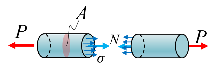
Consider a bar loaded along its axis with a force \(P\), as shown in Figure 8.3.1. To find out what happens inside, we cut the bar perpendicular to its axis and draw a free body diagram of either half. The cut exposes the internal force that the removed half used to exert on the half we kept, and equilibrium of the remaining piece requires
\[
P = N
\]
where \(N\) is the normal force, defined positive when it points out of the cut surface.
Figure 8.3.1: A bar loaded along its axis, cut perpendicular to the load.
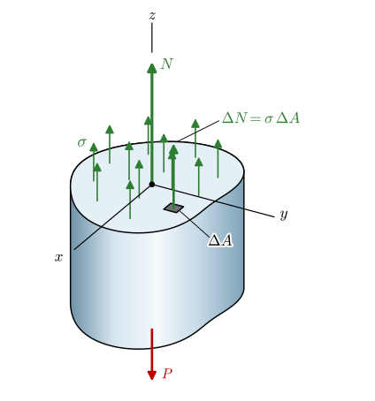
The normal force is a resultant. It is what remains after we add up the infinitely many small forces that the material transmits across every point of the cut surface. Writing that sum as an integral over the cross-sectional area \(A(x)\) gives
\[
N(x) = \int_{A(x)} \sigma(x)\, dA
\tag{8.3.1}\]
which defines the normal stress\(\sigma\) as the intensity with which the internal force is distributed over the surface. Reading 8.3.1 pointwise, the stress at a point on the cut is
and if the distribution is uniform over the cross section, which is the case for a prismatic bar loaded far from its ends, the integral collapses to the average
\[
\boxed{\sigma = \frac{N}{A}}
\tag{8.3.2}\]
With \(A\) measured in \(\text{mm}^2\) and \(N\) in newtons, the stress comes out in \(\text{N}/\text{mm}^2\), which is the megapascal, \(\text{MPa}\). This unit is worth committing to memory because it makes the numbers in engineering practice come out in a comfortable range: structural steel yields somewhere around \(350~\text{MPa}\), and a load of \(1~\text{kN}\) on a square centimetre gives \(10~\text{MPa}\).
Figure 8.3.2: The internal force distributed over the cut surface as a stress.
A cut and a free body diagram therefore always give us the same pair of equations, one from equilibrium and one from the definition of stress,
and the whole of this chapter consists of applying that pair to increasingly interesting geometry.
The sign of the stress carries physical meaning. A positive \(\sigma\) pulls the material apart and is called tensile stress; a negative \(\sigma\) pushes it together and is called compressive stress. Most engineering materials respond quite differently to the two, which is why the sign must be tracked and not discarded along with the magnitude.
When is the stress too high?
Computing a stress is only half of a design task. The other half is deciding whether the number we obtained is acceptable, and that requires a material limit to compare against. The limit we use most often is the yield stress\(\sigma_y\), the stress at which the material stops springing back to its original shape and begins to deform permanently. Below the yield stress the material is in its elastic region, where removing the load removes the deformation. Above it the deformation is plastic and stays. We obtain \(\sigma_y\) experimentally from a tensile test, which we examine in detail in Chapter 8.6.
Designing exactly at the yield stress would leave no room for the things we did not model: a load slightly larger than expected, a batch of material slightly weaker than specified, a hole drilled where the drawing did not show one. We therefore introduce a factor of safety\(\eta\) and design against the allowable stress
so that a factor of \(\eta = 1.5\) means the structure carries half again as much load as it is asked to before yielding begins. The choice of \(\eta\) is a matter of engineering judgment and industry practice rather than mathematics, and it grows with the consequences of failure and with our uncertainty about the loads.
Example 1: Dimensioning a rod
The maximum allowable stress for a material is \(150~\text{MPa}\), and a rod must carry \(8~\text{kN}\) of tensile load. What is the smallest diameter, in whole millimetres, that we can use?
We have one equation and one unknown. The stress is the load over the area, and the area of a circular section of diameter \(d\) is \(\pi(d/2)^2\), so
\[
\sigma_{\max} = \frac{N}{\pi (d/2)^2}
\]
which we solve for \(d\) symbolically before putting any numbers in.
Code
N, sigma_max, d = sp.symbols('N sigma_max d', positive=True)A_circ = sp.pi * (d/2)**2d_sol = sp.solve(sp.Eq(sigma_max, N/A_circ), d)[0]d_num = d_sol.subs({N: 8000, sigma_max: 150})ltx(r"d &=", d_sol, r"\\ d &=", d_num.evalf(4), r"~\text{mm}", aligned=True)
\[ \begin{aligned}d &=\dfrac{2 \sqrt{N}}{\sqrt{\pi} \sqrt{\sigma_{max}}}\\ d &=8.24~\text{mm}\end{aligned} \]
The exact answer is \(8.24~\text{mm}\), and here the rounding must be done with some care. Rounding to the nearest whole millimetre would give \(d = 8~\text{mm}\), and the resulting stress would be
which exceeds the allowable stress. Dimensioning is not ordinary arithmetic: we always round in the direction that adds material. Choosing \(d = 9~\text{mm}\) brings the stress down to \(126~\text{MPa}\), and the factor of safety relative to the allowable stress becomes
Code
eta =150/ sigma_of_d.subs(d, 9)ltx(r"\eta = \frac{\sigma_{\text{allow}}}{\sigma} =", eta.evalf(), precision=3)
so the finished design carries about 19% more load than required before reaching the allowable stress. Note that this margin sits on top of whatever factor of safety was already used to arrive at the \(150~\text{MPa}\) allowable value.
Example 2: A bar with two cross sections
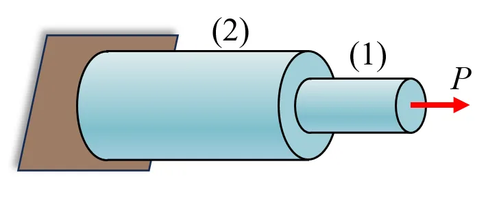
A bar is made up of two segments with different cross sections, as shown in Figure 8.3.3. The first has area \(A_1 = 100~\text{mm}^2\) and the second \(A_2 = 2A_1\). The bar is pulled with \(P = 10~\text{kN}\). Determine the stress in both parts and identify which one is worse off.
Figure 8.3.3: A bar with two different cross sections under a tensile load.
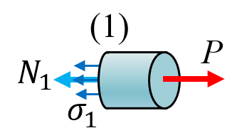
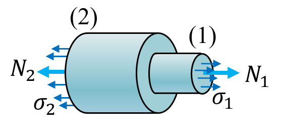
Two cuts are needed, one through each segment, and each gives a free body diagram whose equilibrium determines the normal force in that segment.
Figure 8.3.4: Cut through segment 1
Figure 8.3.5: Cut through segment 2
The first free body is segment 1 cut off from the rest, and the second is the piece of the bar between the two cuts. With the direction to the right positive and each normal force drawn positive in tension, pointing out of its cut face, their equilibrium reads
The narrow segment carries \(100~\text{MPa}\) and the wide one \(50~\text{MPa}\). Both segments transmit the same force, since any cut through the bar exposes the same \(P\), so the stress is inversely proportional to the area alone. Doubling the area halves the stress, and the thin part is always the critical one in a bar of this kind.
The pattern used here is worth keeping. Rather than eliminating unknowns by hand, we write down every relation we know, equilibrium equations and definitions and data alike, and solve them as one system. The bookkeeping is the computer’s job.
Example 3: Several external forces
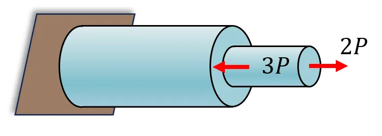
The same bar is now loaded at three points, as shown in Figure 8.3.6. Determine the stresses in the two segments.
Figure 8.3.6: A stepped bar loaded at three points.
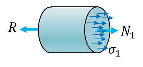
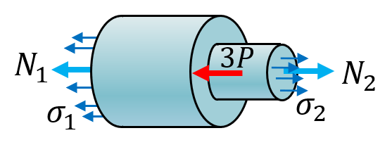
With loads applied in the interior, a single cut no longer suffices. We need one cut per segment, which produces three free bodies, and each contributes an equilibrium equation.
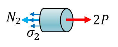
Figure 8.3.7: Left piece, cut once
Figure 8.3.8: Middle piece, cut twice
Figure 8.3.9: Right piece, cut once
With the direction to the right positive and each normal force drawn positive in tension, pointing out of its cut face, the three free bodies give
\[ \begin{aligned}
N_{1} &= - P \\[9.0pt]
N_{2} &= 2 P \\[9.0pt]
R &= - P \\[9.0pt]
\sigma_{1} &= - \dfrac{P}{A_{1}} \\[9.0pt]
\sigma_{2} &= \dfrac{2 P}{A_{2}}
\end{aligned} \]
The first segment ends up in compression, \(\sigma_1 = -P/A_1\), even though the bar as a whole is being pulled. The interior load at the step is large enough to reverse the sign of the internal force upstream of it. The largest stress in magnitude is \(2P/A_2\) in the second segment, so that is where the bar will fail, but a designer who ignored the sign in segment 1 would miss that this part is a candidate for buckling rather than for tensile failure.
Example 4: Stress in a thin-walled cylinder
It is barbecue season, which as always is a good time for structural analysis. A sausage on the grill splits along its length, never around its circumference. Why?
Figure 8.3.10: A sausage, modelled as a thin-walled pressure vessel.
We model the sausage as a thin-walled cylinder of length \(L\), radius \(R\) and wall thickness \(t\), with \(t \ll R \ll L\), filled with an internal pressure \(p\). Use cylindrical coordinates with \(\varphi\) tangential, \(r\) radial and \(z\) axial. The skin is thin enough that we may treat the stress as constant through the wall.
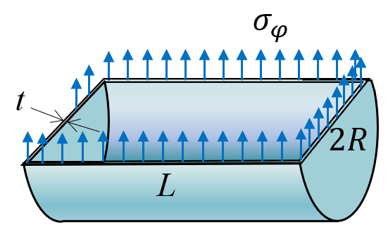
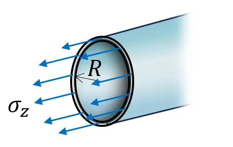
Two cuts are needed because the wall carries stress in two independent directions. Cutting the cylinder lengthwise exposes the hoop stress\(\sigma_\varphi\), which acts tangentially and resists the pressure trying to open the cylinder along its axis. Cutting it across exposes the axial stress\(\sigma_z\), which resists the pressure pushing the two end caps apart.
Figure 8.3.11: The lengthwise cut exposes \(\sigma_\varphi\)
Figure 8.3.12: The transverse cut exposes \(\sigma_z\)
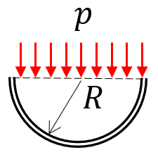
Figure 8.3.13: The pressure acts on the projected width \(2R\)
For the lengthwise cut, the pressure acts on the projected area \(2RL\) and is resisted by two wall strips of area \(tL\) each. For the transverse cut, the pressure acts on the circular area \(\pi R^2\) and is resisted by the annular wall area \(2\pi R t\). The two equilibrium equations are therefore
sigma_varphi, sigma_z, t, L, R_c, p = sp.symbols('sigma_varphi sigma_z t L R p', positive=True)eqs = [sp.Eq(sigma_varphi *2*t*L - p *2*R_c*L, 0), sp.Eq(sigma_z *2*sp.pi*R_c*t - p * sp.pi*R_c**2, 0)]sol = sp.solve(eqs, [sigma_varphi, sigma_z], dict=True)[0]sol | la
The hoop stress is twice the axial stress, \(\sigma_\varphi = 2\sigma_z\), and the ratio is independent of both the length and the pressure. A thin-walled cylinder always carries twice as much stress around its circumference as along its axis, so it tears along a line parallel to its axis.
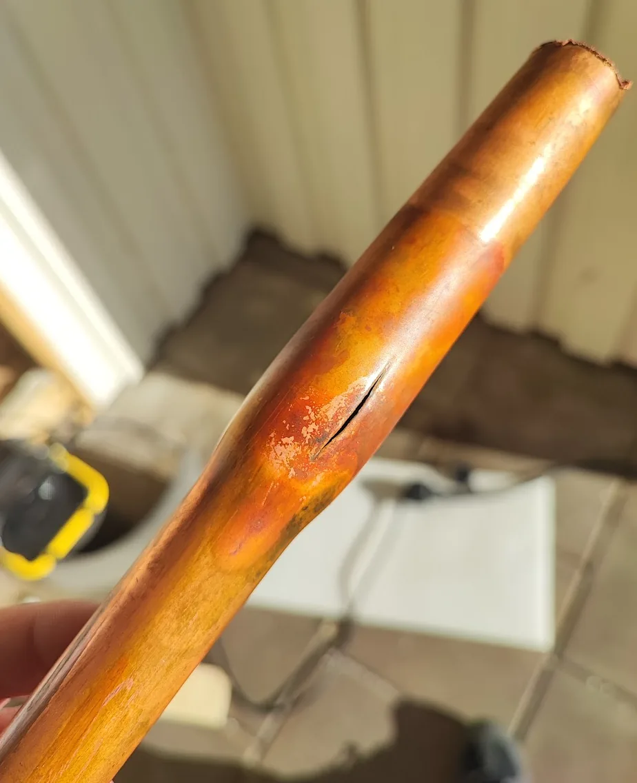
The prediction is easy to confirm outside the kitchen, and the confirmation can be expensive. Water is one of the few substances that expands when it freezes, by roughly nine percent, and a pipe full of it that is sealed at both ends by ice plugs has nowhere to put the extra volume. The internal pressure rises until the wall fails, and Figure 8.3.14 shows what a copper water pipe in the author’s own house did about it.
Figure 8.3.14: A copper water pipe that burst when the water inside it froze. The split runs along the axis, as \(\sigma_\varphi = 2\sigma_z\) requires.
The wall bulged first, which is the plastic deformation that precedes fracture in a ductile metal, and then opened along a line parallel to the axis. Not around the circumference, which the axial stress would have caused had it been the larger of the two, and not at a random angle. The failure is exactly where 8.3.2 applied to the two cuts says it should be.
The lesson has a practical half. A frozen pipe does not leak while it is frozen, because the ice that split it also plugs it. The water arrives when it thaws, usually while nobody is watching, and the resulting damage costs far more than the pipe. Drain the outdoor circuits before winter, insulate what cannot be drained, and check that your insurance is in order.
Example 5: A bar supported by a rod
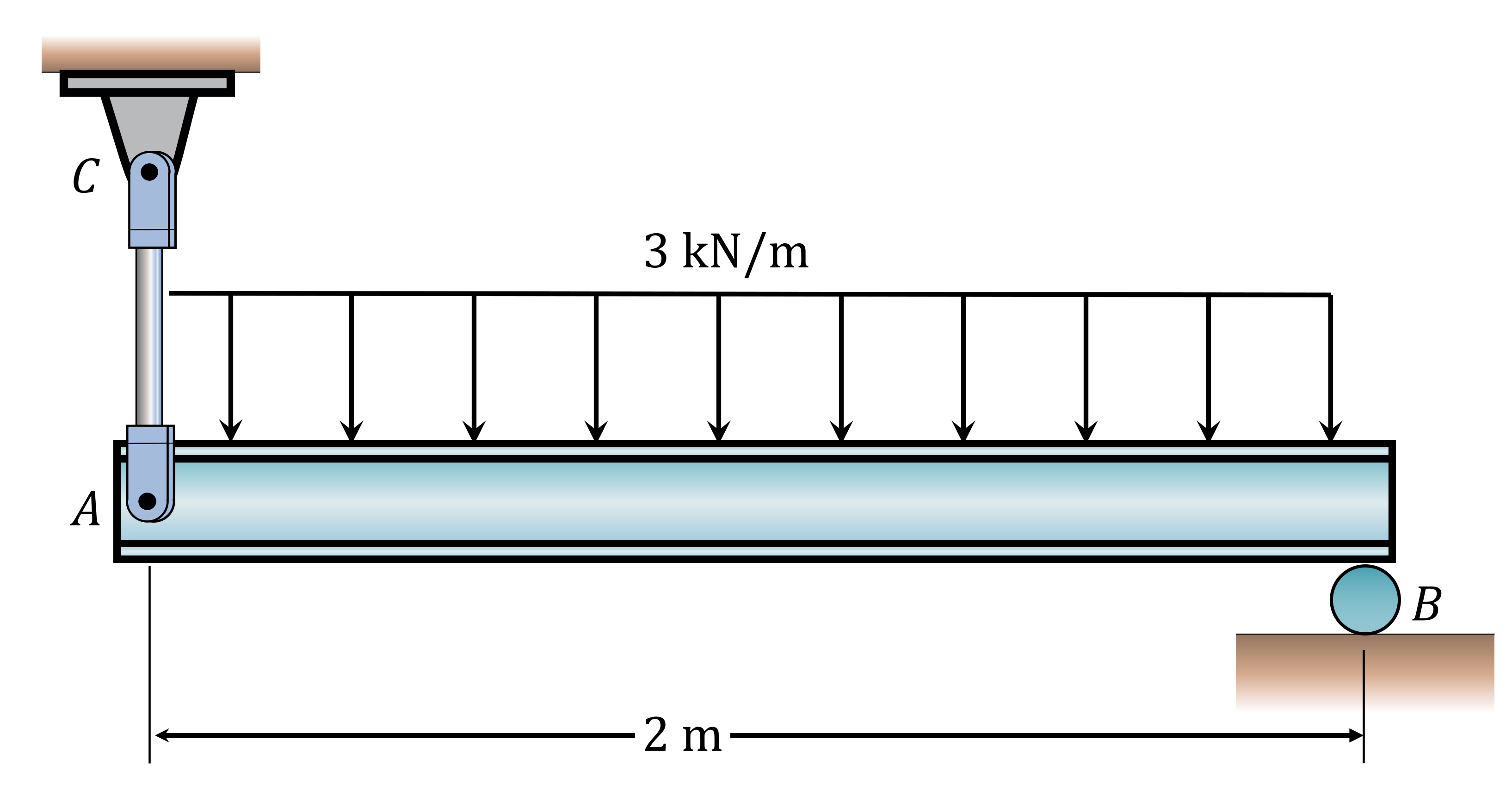
The uniform bar \(AB\) in Figure 8.3.15 has a mass of \(400~\text{kg}\), is supported by a steel rod \(AC\) and a roller at \(B\), and carries a distributed load of \(3~\text{kN}/\text{m}\) over its length. The yield stress of the rod material is \(345~\text{MPa}\) and the factor of safety is \(1.2\). Determine the required diameter of the rod.
Figure 8.3.15: A uniform bar supported by a rod and a roller.
The rod is a two-force member, so the stress in it follows from 8.3.2 once we know the force it carries. Finding that force is a statics problem, and the free body diagram of the bar is where it starts.
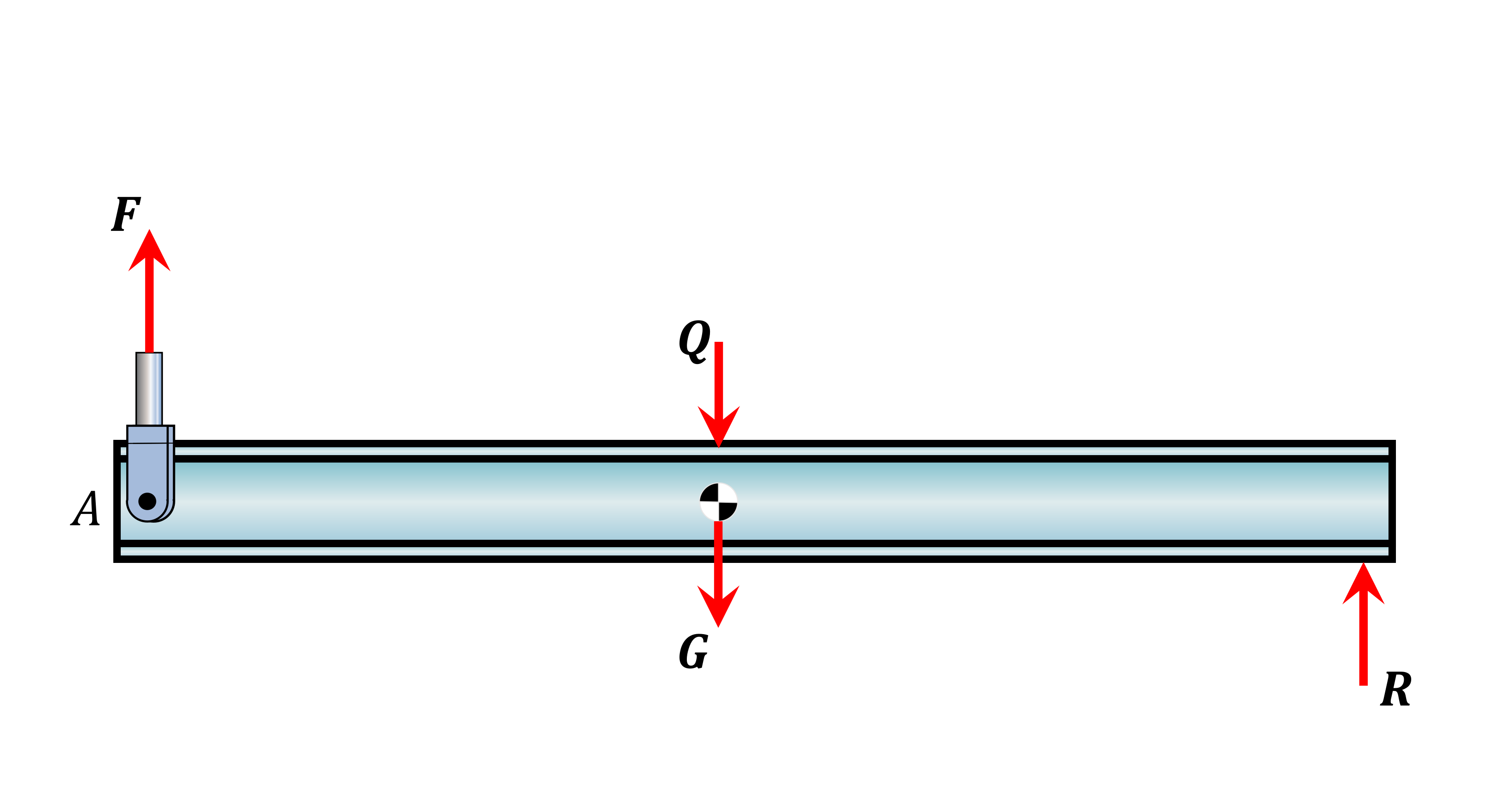
Figure 8.3.16: Free body diagram of the bar.
The distributed load is replaced by a resultant \(Q\) acting at its centroid, and the weight \(G = mg\) acts at the centre of the uniform bar. The bar has length \(\ell = 2~\text{m}\), so
Both resultants act at \(\ell/2\) from \(B\), which makes the moment equation short. With upward forces and counterclockwise moments positive, vertical equilibrium and moment equilibrium about \(B\) read
\[
\begin{aligned}
F - Q - G + R &= 0 \\
(Q + G)\,\frac{\ell}{2} - F\ell &= 0
\end{aligned}
\]
and the moment equation alone gives \(F = (Q + G)/2\).
Code
F, R = sp.symbols('F R', real=True)ell =2# length of the bar [m]Q =3e3* ell # 3 kN/m over the barG =400*9.82# weight of the bareqs = [sp.Eq(F - Q - G + R, 0), # vertical equilibrium sp.Eq((Q + G)*ell/2- F*ell, 0)] # moments about Bsol = sp.solve(eqs, [F, R], dict=True)[0]sol | la
\[ \begin{aligned}
F &= 4964.0 \\[9.0pt]
R &= 4964.0
\end{aligned} \]
The rod carries \(F = 4964~\text{N}\). With a yield stress of \(345~\text{MPa}\) and a factor of safety of \(1.2\), the allowable stress follows from 8.3.3, and the required diameter follows from setting the actual stress in the rod equal to it,
d = sp.symbols('d', positive=True)sigma_allow =345/1.2d_req = sp.solve(sp.Eq(sigma_allow, sol[F] / (sp.pi*(d/2)**2)), d)[0]ltx(r"\sigma_{\text{allow}} &=", sigma_allow, r"~\text{MPa}",r"\\ d &=", d_req.evalf(), r"~\text{mm}", aligned=True, precision=4)
\[ \begin{aligned}\sigma_{\text{allow}} &=287.5~\text{MPa}\\ d &=4.689~\text{mm}\end{aligned} \]
Rounding upward as always, the rod needs a diameter of at least \(5~\text{mm}\). Whether such a slender rod is a sensible piece of hardware is a separate question: it satisfies the stress requirement, but a designer would also check that it is stiff enough, that it can be attached to anything, and that it will not be damaged by handling.
Example 6: A pillar under its own weight
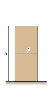
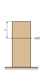
A pillar of height \(H\) and cross-sectional area \(A\) stands on the floor, as shown in Figure 8.3.17. It is made of a homogeneous material with density \(\rho\). Determine the stress in the pillar as a function of the depth below its top.
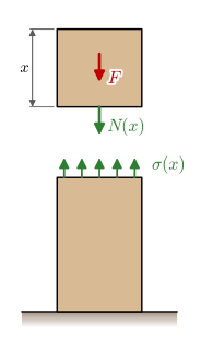
The only load is the pillar’s own weight, which is spread through its volume, so every cut carries a different normal force. We let the coordinate \(x\) run downward from the top and cut the pillar at \(x\), Figure 8.3.18. The upper piece has length \(x\) and weight \(F\). On its cut face the normal force \(N(x)\) is drawn positive, pointing out of the face and therefore downward, Figure 8.3.19.
Figure 8.3.17: The pillar. The dashed line marks a cross section of area \(A\).
Figure 8.3.18: A cut at depth \(x\) below the top.
Figure 8.3.19: The two pieces. \(N(x)\) is the resultant of the stress \(\sigma(x)\) over the cut.
Equilibrium of the upper piece in the downward direction, the geometry of that piece, and the definition of stress give
\[
\left\lbrace \begin{array}{ll}
N + F = 0, \quad F = mg & \text{equilibrium}\\[4pt]
m = \rho V, \quad V = Ax & \text{geometry}\\[4pt]
\sigma = \dfrac{N}{A} & \text{stress}
\end{array}\right.
\]
which is five equations in the five unknowns \(N\), \(F\), \(\sigma\), \(m\) and \(V\). As in Example 2, we hand the whole set to SymPy.
Code
N, F, sigma, m, V = sp.symbols('N F sigma m V', real=True)rho, g, A, x = sp.symbols('rho g A x', positive=True)eqs = [sp.Eq(N + F, 0), sp.Eq(F, m*g), # equilibrium, downward positive sp.Eq(m, rho*V), sp.Eq(V, A*x), # the upper piece sp.Eq(sigma, N/A)] # stress in the cutsol = sp.solve(eqs, [N, F, sigma, m, V], dict=True)[0]sol | la
\[ \begin{aligned}
F &= A g \rho x \\[9.0pt]
N &= - A g \rho x \\[9.0pt]
V &= A x \\[9.0pt]
m &= A \rho x \\[9.0pt]
\sigma &= - g \rho x
\end{aligned} \]
The stress is
\[
\sigma(x) = -\rho g x
\]
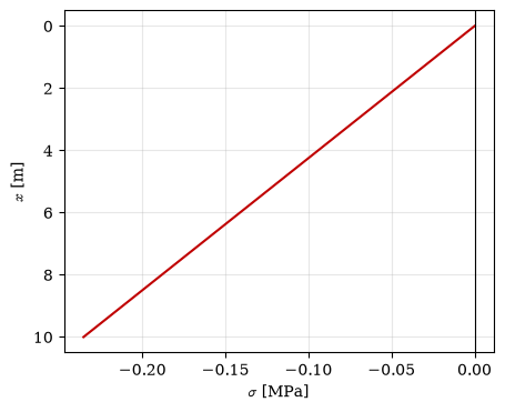
and it is negative, so the pillar is in compression, as we would expect. It grows linearly from zero at the top to \(-\rho g H\) at the floor. The area has dropped out: a wider pillar carries more weight above every cut, and that weight is spread over a proportionally larger section. A dimension check never hurts,
For a concrete pillar with \(\rho = 2400~\text{kg/m}^3\) and \(H = 10~\text{m}\), the stress at the floor is \(\sigma(H) = -2400 \cdot 9.81 \cdot 10~\text{Pa} = -0.235~\text{MPa}\). Figure 8.3.20 shows the distribution with \(x\) pointing down, as in the pillar.
Code
vals = {rho: 2400, g: 9.81}H =10sigma_MPa = sp.lambdify(x, sol[sigma].subs(vals) /1e6)x_vals = np.linspace(0, H, 50)fig, ax = plt.subplots(figsize=(5, 4))ax.plot(sigma_MPa(x_vals), x_vals, color='#c00000')ax.axvline(0, color='k', lw=0.8)ax.invert_yaxis() # x runs downward, as in the pillarax.set(xlabel=r'$\sigma$[MPa]', ylabel='$x$ [m]')ax.grid(alpha=0.3)plt.show()
Figure 8.3.20: The stress in a 10 m concrete pillar. It is zero at the top and most compressive at the floor.
The stresses are small, which raises the question of how tall the pillar may be before the concrete at its base is crushed. Setting the stress at the floor equal to the compressive strength \(\sigma_c\) gives
Self-weight alone limits a concrete pillar to well over a kilometre, which is why it rarely governs the design of buildings, where the floors and everything on them weigh far more than the columns. It does matter for tall masonry towers, deep mine shafts with hanging cables, and anywhere else the structure itself is most of the load.
Saint-Venant’s principle
Every example in this chapter took the stress to be \(N/A\) on every cut, although the loads entered through pins, clamps and supports. Close to such a point the assumption is false. A force pressed onto a small patch of the end face of a bar gives a large stress under the patch and almost none at the corners of the face. A little farther along the bar the stress has spread out, and a few widths away it is uniform.
Saint-Venant made this observation general in his 1855 memoir on the torsion of prisms [1]. Two load distributions with the same resultant force and moment produce stress fields that differ appreciably only within a distance of about the largest dimension of the cross section from where they act. Beyond that distance the stress depends on the resultant alone. The principle is an empirical rule, confirmed by experiment and by every exact solution we have, and it carries each model in this book that replaces a real load by its resultant. The rod, the beam and the shaft are accurate from about one section depth away from supports, load points and changes of section, and not closer. The same rule applies to a hole or a notch, whose disturbance dies out over a distance of the order of its own size, as Chapter 8.20 shows.
Looking ahead
Everything in this chapter rests on one assumption that we never stated explicitly: that the stress is uniform across the cut. That assumption fails near holes, near sharp corners, near points where load is introduced, and everywhere in a bent or twisted member. Removing it requires the stress to become a field that varies from point to point, and requires us to admit that a cut in a different direction exposes a different stress. Those two steps take us from the scalar \(\sigma = N/A\) to the stress tensor, which is the subject of Chapter 8.7. Before that we need the companion notion to stress, which measures deformation rather than force.
Problems
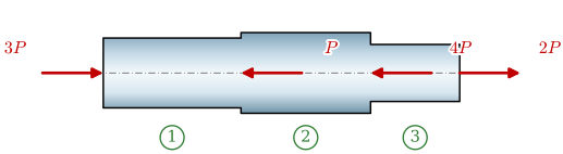
Exercise 8.3.1 A straight bar is made of three cylindrical parts with cross-sectional areas \(A_1 = 75~\text{mm}^2\), \(A_2 = 100~\text{mm}^2\) and \(A_3 = 50~\text{mm}^2\), loaded as shown in Figure 8.3.21. Determine the nominal stress in each part for \(P = 2~\text{kN}\). What are the stresses at the steps between the parts if these are made with a fillet radius \(r = 1.5~\text{mm}\)? The stress concentration factors are found in Chapter 8.20.
Figure 8.3.21: A stepped bar of three cylindrical parts under four axial loads.
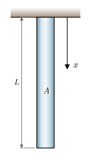
Exercise 8.3.2 A straight homogeneous bar of total mass \(M\), length \(L\) and cross-sectional area \(A\) hangs freely from one end, Figure 8.3.22. Its own weight gives rise to a normal stress in the bar. Use the method of sections to determine the normal stress in a cross section at the distance \(x\) from the point of suspension, and check the result against the special cases \(x = 0\) and \(x = L\).
Figure 8.3.22: A bar hanging freely under its own weight.
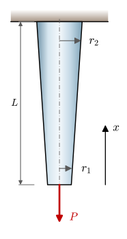
Exercise 8.3.3 Determine the stress \(\sigma(x)\) in the slightly conical bar of length \(L\) in Figure 8.3.23. The cross section is circular, with radius \(r_1\) at \(x = 0\) and \(r_2\) at \(x = L\), and the bar carries the force \(P\) at its lower end.
Figure 8.3.23: A slightly conical bar hanging from the ceiling, loaded by a force at its lower end.
References
[1]
Saint-Venant AJCB de. Mémoire sur la torsion des prismes. Mémoires Présentés Par Divers Savants à l’Académie Des Sciences de l’Institut Impérial de France 1855;14:233–560.