Strain energy

A body loaded slowly from zero stores the work of the loads as strain energy, which an elastic body gives back on unloading. We compute it from the continuum model of Hooke’s law in 3D. A small cube of material whose strain grows by \(d\bm\varepsilon\) receives the work \(\bm\sigma : d\bm\varepsilon = \sigma_{ij}\,d\varepsilon_{ij}\) per unit volume. For a linear elastic material \(\bm\sigma\) grows in proportion to \(\bm\varepsilon\), so the integral from zero is half the product of the final values, the strain energy density

\[ \mathcal{W} = \tfrac{1}{2}\,\bm\sigma : \bm\varepsilon , \qquad U = \int_\Omega \mathcal{W}\,dV . \tag{8.17.1}\]

The rod, the shaft and the beam each impose a kinematic assumption on the continuum, and 8.17.1 reduces with them. In the rod of The rod equation only \(\sigma_x = E\varepsilon_x\) with \(\varepsilon_x = du/dx\) remains, uniform over the cross-section, and the normal force is \(N = EA\,du/dx\). In the shaft of Torsion only the shear stress \(\tau = G\gamma\) remains, with \(\gamma = \rho\,d\theta/dx\) growing with the radius \(\rho\), and the torque is \(M_t = GJ\,d\theta/dx\). In the beam of Beam theory only \(\sigma_x = E\varepsilon_x\) remains, with \(\varepsilon_x = -y\,w''\) from the displacement field 8.16.3, and the bending moment is \(M = EI\,w''\). Integrating \(\mathcal{W}\) over the cross-section first and along the axis second gives

x, y, rho, E, G, A, I, J = sp.symbols('x y rho E G A I J', positive=True)
up, thp, wpp = sp.symbols(r"u' \theta' w''", real=True)
# energy per unit length: the density integrated over the cross-section
rod = sp.Rational(1, 2)*E*up**2*A                                   # sigma*eps/2 = E u'^2/2, uniform over A
shaft = sp.Rational(1, 2)*G*thp**2*J                                # G (rho theta')^2/2 over the section: J = int rho^2 dA
beam = sp.Rational(1, 2)*E*wpp**2*I                                 # E (y w'')^2/2 over the section: I = int y^2 dA
N, Mt, M = sp.symbols('N M_t M', real=True)

where \(u'\), \(\theta'\) and \(w''\) are the strain measures of the three models, and the second forms follow from \(N = EAu'\), \(M_t = GJ\theta'\) and \(M = EIw''\). The strain energy of a structure is the sum over its members,

\[ U = \int\frac{N^2}{2EA}\,dx + \int\frac{M_t^2}{2GJ}\,dx + \int\frac{M^2}{2EI}\,dx . \tag{8.17.2}\]

We write the torque as \(M_t\) in this chapter to keep it apart from the bending moment \(M\). The shear force of a beam also stores energy; for slender beams it is small against the bending term, and we leave it out.

Internal virtual work and virtual displacements

Give a deformable body a virtual displacement \(\delta\bm u\), allowed by the supports. The loads do the external virtual work \(\delta W_{\text{ext}}\), and the stresses do the internal virtual work on the virtual strain \(\delta\bm\varepsilon\) that \(\delta\bm u\) causes,

\[ \delta W_{\text{int}} = \int_\Omega \bm\sigma : \delta\bm\varepsilon\,dV . \]

The principle of virtual displacements for a deformable body states that it is in equilibrium if and only if

\[ \delta W_{\text{int}} = \delta W_{\text{ext}} \quad\text{for every allowed } \delta\bm u . \tag{8.17.3}\]

For the rod of The rod equation, fixed at \(x = 0\), loaded by the distributed load \(f\) and the end force \(F\) at \(x = L\), 8.17.3 reads

\[ \int_0^L N\,\delta u'\,dx = \int_0^L f\,\delta u\,dx + F\,\delta u(L) , \qquad \delta u(0) = 0 . \tag{8.17.4}\]

Integrating the left side by parts gives \(\bigl[N\delta u\bigr]_0^L - \int_0^L N'\,\delta u\,dx\). The term at \(x = 0\) vanishes because the support does not move, and what remains is

\[ \int_0^L\bigl(-N' - f\bigr)\delta u\,dx + \bigl(N(L) - F\bigr)\delta u(L) = 0 . \]

Since \(\delta u\) is arbitrary inside the rod and at its end, both brackets vanish: \(-N' = f\), which is 8.12.1, and \(N(L) = F\), the natural boundary condition of 8.12.5. The principle of virtual displacements contains the differential equation and its force boundary condition, and the displacement boundary condition enters as the requirement that \(\delta u\) vanishes at the support. Read from right to left, the same integration by parts turns the differential equation into 8.17.4, which is the weak form of the finite element method; the arbitrary function there is this virtual displacement.

Castigliano’s first theorem

A structure loaded by forces \(P_i\) at points that move by \(\Delta_i\) in the directions of the forces has its strain energy as a function of these displacements, \(U(\Delta_1, \Delta_2, \dots)\). A virtual displacement that changes only \(\Delta_i\) does the external work \(P_i\,\delta\Delta_i\) and increases the strain energy by \(\delta U = (\partial U/\partial\Delta_i)\,\delta\Delta_i\), which is the internal virtual work. 8.17.3 for each \(i\) gives Castigliano’s first theorem,

\[ P_i = \frac{\partial U}{\partial\Delta_i} . \tag{8.17.5}\]

Equivalently, the total potential energy \(\Pi = U - \sum_i P_i\Delta_i\) is stationary at equilibrium, \(\partial\Pi/\partial\Delta_i = 0\), and for a stable structure it is a minimum. When \(U\) is a quadratic form in the displacements, \(U = \tfrac12\bm\Delta^\mathsf{T}\bm K\bm\Delta\), 8.17.5 is the linear system \(\bm K\bm\Delta = \bm P\), and the stiffness matrix is the matrix of second derivatives of the strain energy, \(K_{ij} = \partial^2 U/\partial\Delta_i\,\partial\Delta_j\).

Example 1: A two-bar truss by Castigliano’s first theorem

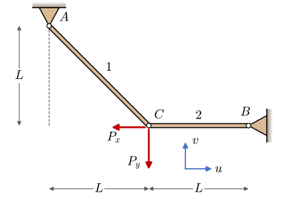
Two steel bars, \(E = 210\) GPa and \(A = 100\) mm², meet at the joint \(C\) (Figure 8.17.1). Bar 1 runs to the pin \(A\) at \(45^\circ\), bar 2 runs horizontally to the pin \(B\), with \(L = 1\) m. The joint carries the load \(P_x = -3\) kN, \(P_y = -10\) kN. Find the displacement of \(C\) and the forces in the bars.

The joint has two degrees of freedom, \(u\) and \(v\) along \(x\) and \(y\). A bar \(e\) with the stiffness \(k_e = EA/\ell_e\) and the unit vector \(\bm e_e\) from its support to \(C\) lengthens by \(\bm e_e\cdot[u,\ v]^\mathsf{T}\), so the strain energy of the truss is

\[ U(u, v) = \sum_{e=1}^{2}\tfrac{1}{2}k_e\bigl(\bm e_e\cdot[u,\ v]^\mathsf{T}\bigr)^2 , \qquad \bm e_1 = \tfrac{1}{\sqrt 2}\begin{bmatrix}1\\-1\end{bmatrix} , \quad \bm e_2 = \begin{bmatrix}-1\\0\end{bmatrix} , \]

and 8.17.5 gives the two equations \(\partial U/\partial u = P_x\), \(\partial U/\partial v = P_y\). The bar forces follow from the elongations, \(N_e = k_e\,\bm e_e\cdot[u,\ v]^\mathsf{T}\).

u, v = sp.symbols('u v', real=True)
Ev, Av, Lv = 210e9, 100e-6, 1.0
bars = {1: (np.array([1, -1])/np.sqrt(2), Lv*np.sqrt(2)), 2: (np.array([-1.0, 0.0]), Lv)}
U_t = sum(Ev*Av/l/2*(e[0]*u + e[1]*v)**2 for e, l in bars.values())
P = {u: -3e3, v: -10e3}
d = sp.solve([sp.diff(U_t, u) - P[u], sp.diff(U_t, v) - P[v]], [u, v])
K_energy = np.array(sp.hessian(U_t, (u, v)), dtype=float)
K_assembled = sum(Ev*Av/l*np.outer(e, e) for e, l in bars.values())   # the truss element of Systematic truss analysis
N_bar = {b: Ev*Av/l*(e[0]*float(d[u]) + e[1]*float(d[v])) for b, (e, l) in bars.items()}

Solving the two equations, the displacement of the joint, the bar forces, and the stiffness matrix as the second derivative of \(U\) against the matrix assembled from the truss elements of Systematic truss analysis are

The joint moves 1.97 mm down and 0.62 mm to the left, and both bars are in tension, bar 1 with 14.14 kN and bar 2 with 13.0 kN. This truss is statically determinate, so the bar forces could also have come from the equilibrium of the joint, \(N_1/\sqrt2 = 10\) kN and \(N_2 = 3 + 10\) kN, which they match. The energy route gave the displacement as well, and its stiffness matrix is the assembled truss matrix of Systematic truss analysis: the matrix there is the second derivative of the strain energy. That is how a finite element program builds its stiffness matrix, element by element, from the energy of each element.

Virtual forces and Castigliano’s second theorem

The second principle swaps the roles. Instead of a virtual displacement of the real structure, take a virtual force system: any set of loads \(\delta P_i\) with internal forces \(\delta N\), \(\delta M_t\), \(\delta M\) that are in equilibrium with them. Its virtual work on the real, compatible deformation is the same whether computed at the loads or inside the members,

\[ \sum_i\delta P_i\,\Delta_i = \int\delta N\,\frac{N}{EA}\,dx + \int\delta M_t\,\frac{M_t}{GJ}\,dx + \int\delta M\,\frac{M}{EI}\,dx , \tag{8.17.6}\]

since \(N/EA\), \(M_t/GJ\) and \(M/EI\) are the real strain measures. This is the principle of virtual forces. It expresses that the deformation is compatible, while the principle of virtual displacements expresses that the forces are in equilibrium.

Two forms of 8.17.6 are used. If the virtual force system is the real one varied by \(\delta P_i\), then \(\delta N = (\partial N/\partial P_i)\,\delta P_i\) and so on, the right side is \((\partial U/\partial P_i)\,\delta P_i\), and

\[ \Delta_i = \frac{\partial U}{\partial P_i} , \qquad \theta_i = \frac{\partial U}{\partial M_i} . \tag{8.17.7}\]

This is Castigliano’s second theorem: the displacement of the point where a force acts, in the direction of the force, is the derivative of the strain energy with respect to that force, and the rotation where a moment acts is the derivative with respect to the moment. Strictly the derivative is of the complementary energy, which equals \(U\) for a linear elastic structure. To find the displacement of a point where no force acts, add a dummy force there, differentiate, and set it to zero.

If instead the virtual force system is a single unit force at the point and in the direction of the wanted displacement, with the internal forces \(n\), \(m_t\) and \(m\), 8.17.6 becomes the unit-load method,

\[ \Delta = \int\frac{nN}{EA}\,dx + \int\frac{m_t M_t}{GJ}\,dx + \int\frac{mM}{EI}\,dx . \]

For a linear structure \(n = \partial N/\partial P\), so the two forms are the same calculation.

Example 2: The tip of a cantilever

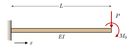
A cantilever of length \(L\) and bending stiffness \(EI\) carries the force \(P\) at its free end (Figure 8.17.2). Find the deflection and the rotation of the tip.

No moment acts at the tip, so we add a dummy moment \(M_0\) there. Cutting the beam at \(x\) and taking moments of the part to the right, the bending moment is

\[ M(x) = -P\,(L - x) - M_0 , \]

and the strain energy is \(U = \int_0^L M^2/(2EI)\,dx\). By 8.17.7 the tip deflection along \(P\) and the tip rotation along \(M_0\) are

\[ \delta = \frac{\partial U}{\partial P}\bigg|_{M_0 = 0} , \qquad \theta = \frac{\partial U}{\partial M_0}\bigg|_{M_0 = 0} . \]

P_, M0, L_, EI = sp.symbols('P M_0 L EI', positive=True)
M_x = -P_*(L_ - x) - M0
U_c = sp.integrate(M_x**2/(2*EI), (x, 0, L_))
delta_tip = sp.simplify(sp.diff(U_c, P_).subs(M0, 0))
theta_tip = sp.simplify(sp.diff(U_c, M0).subs(M0, 0))

Differentiating and setting \(M_0 = 0\),

These are the tip deflection and slope of a cantilever in every handbook, obtained here without solving the elastic line. The sign of \(M\) does not matter, because \(U\) contains \(M^2\); the deflection comes out in the direction of \(P\), down, and the rotation in the direction of \(M_0\).

Example 3: The deflection of a helical spring

The helical compression spring of Springs has the wire diameter \(d\), the mean coil diameter \(D\) and \(n\) active coils, and carries the axial force \(F\) (Figure 9.8.9). Cutting the wire anywhere shows the torque \(M_t = FD/2\) about the wire axis; the direct shear force in the wire stores much less energy and is left out. The wire is a shaft of length \(\ell = \pi Dn\) with the polar moment \(J = \pi d^4/32\), so by 8.17.2

\[ U = \frac{M_t^2\,\ell}{2GJ} = \frac{(FD/2)^2\,\pi Dn}{2G\,\pi d^4/32} , \qquad \delta = \frac{\partial U}{\partial F} . \]

F_, D, d_, n, G_ = sp.symbols('F D d n G', positive=True)
U_s = (F_*D/2)**2*sp.pi*D*n/(2*G_*sp.pi*d_**4/32)
delta_s = sp.simplify(sp.diff(U_s, F_))
spring_vals = {F_: 100, D: sp.Rational(32, 1000), d_: sp.Rational(4, 1000), n: 10, G_: sp.Float(79.3e9)}

Castigliano’s second theorem gives the spring deflection, and for a spring with \(d = 4\) mm, \(D = 32\) mm, \(n = 10\) and \(G = 79.3\) GPa under \(F = 100\) N,

This is 9.8.8, which Springs derived from the twist of the wire.

Example 4: A statically indeterminate beam

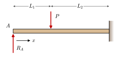
The beam of Example 2 in Beam theory is pinned at \(A\), \(x = 0\), clamped at \(x = L_1 + L_2\), and carries the point load \(P\) at \(x = L_1\) (Figure 8.16.11). It has one support reaction more than equilibrium can determine. We choose the pin reaction \(R_A\) as the unknown, the redundant, remove the pin and apply \(R_A\) as a load instead (Figure 8.17.3). The clamp alone then holds a statically determinate cantilever, whose bending moment follows from the loads \(P\) and \(R_A\),

\[ M(x) = R_A\,x \quad (0 \le x \le L_1) , \qquad M(x) = R_A\,x - P\,(x - L_1) \quad (L_1 \le x \le L_1 + L_2) . \]

The pin does not move, so the displacement of \(A\) in the direction of \(R_A\) is zero, and by 8.17.7

\[ \frac{\partial U}{\partial R_A} = 0 , \]

the compatibility condition that equilibrium could not supply. This form of the second theorem, that a redundant makes the strain energy stationary, is the principle of least work that Menabrea announced in 1858 in the words of the epigraph. His proof did not hold; Castigliano gave the first rigorous one in his thesis of 1873 and his book of 1879.

R_A, L1, L2 = sp.symbols('R_A L_1 L_2', positive=True)
M_1, M_2 = R_A*x, R_A*x - P_*(x - L1)
U_p = sp.integrate(M_1**2/(2*EI), (x, 0, L1)) + sp.integrate(M_2**2/(2*EI), (x, L1, L1 + L2))
R_A_cast = sp.factor(sp.solve(sp.diff(U_p, R_A), R_A)[0])

# check with the elastic line: EI w'' = M, w(0) = 0, w and w' zero at the clamp, w and w' continuous at L1
C1, C2, C3, C4, R = sp.symbols('C_1 C_2 C_3 C_4 R', real=True)
w1 = sp.integrate(sp.integrate(R*x, x), x)/EI + C1*x + C2
w2 = sp.integrate(sp.integrate(R*x - P_*(x - L1), x), x)/EI + C3*x + C4
Lt = L1 + L2
bc = [w1.subs(x, 0), w2.subs(x, Lt), sp.diff(w2, x).subs(x, Lt),
      (w1 - w2).subs(x, L1), sp.diff(w1 - w2, x).subs(x, L1)]
R_A_line = sp.factor(sp.solve(bc, [C1, C2, C3, C4, R], dict=True)[0][R])

Solving \(\partial U/\partial R_A = 0\), and checking against the elastic line \(EIw'' = M\) with the same bending moment, \(w = 0\) at the pin, \(w = w' = 0\) at the clamp and continuity at the load,

With the redundant known, the rest of the beam follows from equilibrium. For the load in the middle, \(L_1 = L_2\), the pin carries \(\tfrac{5}{16}P\) and the clamp the remaining \(\tfrac{11}{16}P\), the values of the handbook.

Displacement method and force method

The two theorems lead to two ways of analysing a structure. The force method takes the redundant forces as unknowns and gets one compatibility equation for each from 8.17.7, as in Example 4. It suits hand calculation of structures with few redundants, but the redundants must be chosen by hand, and the choice differs from structure to structure. The displacement method takes the displacements of the joints as unknowns and gets one equilibrium equation for each from 8.17.5, as in Example 1. Its unknowns follow from the mesh alone, every structure gives a system \(\bm K\bm u = \bm f\) of the same form, and it does not care whether the structure is statically determinate. That is why the finite element method solves for displacements.

The nodal balance as virtual work

Systematic truss analysis solved \(\bm K\bm u = \bm f\), the equilibrium of every node. Read as virtual work, the system says

\[ \delta\bm u^\mathsf{T}\bigl(\bm K\bm u - \bm f\bigr) = 0 \quad\text{for every allowed } \delta\bm u , \]

the internal virtual work \(\delta\bm u^\mathsf{T}\bm K\bm u\) of the bars against the external virtual work \(\delta\bm u^\mathsf{T}\bm f\) of the loads. Choosing a \(\delta\bm u\) that moves only node \(i\), in one direction, picks out one row: the force balance of node \(i\) in that direction. A supported node may not move, so its \(\delta\bm u\) is zero and its reaction never enters, exactly as the reactions dropped out of the mechanisms in Virtual work.

The finite element method keeps this reading and changes the bars into elements of a continuum. A virtual displacement that moves one node, spread over the elements around it by their shape functions, gives the force balance of that node, and the force an element exerts on it is the integral of the stress against the virtual strain, \(\int\bm\sigma : \delta\bm\varepsilon\,dV\) of 8.17.3. The rest of the method is how to build the shape functions and how to integrate.

Further reading

Castigliano’s theorems, the unit-load method and the force method for beams and frames are treated with many examples in chapter 14 of Hibbeler’s Mechanics of Materials [1].