“We denote by A a point of the body whose state is to be considered, and to that end we imagine an infinitely small sphere with centre A cut out of the body. The totality of the stresses on all the surface elements of this sphere constitutes the state of stress at the body point A.”
— Christian Otto Mohr, Abhandlungen aus dem Gebiete der technischen Mechanik, 1906, our translation
Two results from the preceding chapters do not fit into a scalar description. In Chapter 8.4 we found that the same axial load produces different normal and shear stresses depending on the angle of the cut, so a single number cannot be the whole story about the stress at a point. In Chapter 8.5 we found that the strain is the gradient of a displacement field, and once the displacement has more than one component that gradient has more than one entry. Both point to the same conclusion: stress and strain are matrices, not numbers.
This chapter constructs those matrices, derives the equations they satisfy, and shows that the earlier scalar results are what the matrices reduce to in one dimension. Everything that follows in this book, the beam of Chapter 8.16 included, is a special case of what we set up here.
The one-dimensional case as a starting point
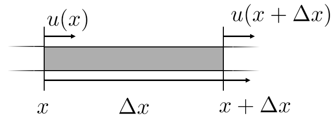
For an infinitesimal element of length \(\Delta x\), the displacement at \(x\) is \(u(x)\) and at the other end \(u(x+\Delta x)\), so the strain is the difference divided by the length,
and the stress follows from Hooke’s law \(\sigma = E\varepsilon\).
Figure 8.7.1: An infinitesimal element in one dimension.
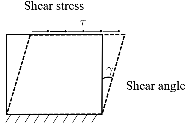
Shear is the other elementary deformation. A shear stress \(\tau\) tilts the element through the shear angle \(\gamma\), and the constitutive relation is \(\tau = G\gamma\).
Figure 8.7.2: Pure shear of an infinitesimal element.
The general state of strain
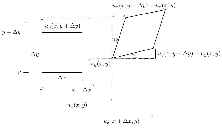
In two dimensions the displacement is a vector field \(\bm u = (u_x, u_y)\) and the element can stretch in two directions while simultaneously shearing. Figure 8.7.3 shows the four independent deformations: two extensions and two contributions to the change of angle.
Figure 8.7.3: The four independent deformations of a two-dimensional element: the two extensions \(\varepsilon_x\) and \(\varepsilon_y\), and the two edge tilts \(\gamma_1\) and \(\gamma_2\) whose sum is the change of the right angle.
Figure 8.7.4: The same element deforming. Both extensions and both tilts happen at once, and each is a difference of displacements divided by the length it acts over.
The extension in the \(x\) direction comes from the variation of \(u_x\) along \(x\), and the extension in the \(y\) direction from the variation of \(u_y\) along \(y\),
The shear contribution is the tilt of an originally vertical or horizontal edge. Moving along \(x\), the vertical displacement changes by \(u_y(x+\Delta x, y) - u_y(x,y)\), and trigonometry gives the tilt angle \(\gamma_1\) of the originally horizontal edge as
Assuming deformations small enough that \(\tan\gamma_1 \approx \gamma_1\), and adding the tilt \(\gamma_2 = \partial u_x/\partial y\) of the originally vertical edge, the total change of the right angle between the two edges is
giving six independent strains in total. Collecting them into a matrix, with the tensor shear strains\(\tfrac{1}{2}\gamma\) off the diagonal, gives the strain tensor
or in direct notation \(\bm\varepsilon = \tfrac{1}{2}\left(\nabla\bm u + \nabla\bm u^\mathsf{T}\right)\), the symmetric part of the displacement gradient. Written out, that gradient is the matrix of every derivative of every displacement component,
with the component differentiated running down the rows and the direction of differentiation across the columns. Nine derivatives go in, and adding the transpose averages each entry with its mirror across the diagonal, which leaves the six independent strains of 8.7.2. Checking a diagonal entry, \(\varepsilon_{11} = \tfrac{1}{2}(\partial u_1/\partial x_1 + \partial u_1/\partial x_1) = \partial u_x/\partial x\), recovers \(\varepsilon_x\). Checking an off-diagonal entry, \(\varepsilon_{12} = \tfrac{1}{2}(\partial u_1/\partial x_2 + \partial u_2/\partial x_1) = \tfrac{1}{2}\gamma_{xy}\), gives half the engineering shear strain.
Remark 8.7.1. The displacement gradient contains something that is not strain. Every matrix splits uniquely into a symmetric and an antisymmetric part,
\[
\nabla\bm u = \underbrace{\tfrac{1}{2}\left(\nabla\bm u + \nabla\bm u^\mathsf{T}\right)}_{\bm\varepsilon} + \underbrace{\tfrac{1}{2}\left(\nabla\bm u - \nabla\bm u^\mathsf{T}\right)}_{\bm\omega}
\tag{8.7.5}\]
and in two dimensions the antisymmetric part has the single entry \(\omega_{xy} = \tfrac{1}{2}(\gamma_2 - \gamma_1)\), an infinitesimal rigid rotation. Rotating a body does not strain it, so strain is what is left once \(\bm\omega\) is removed. The one half is what taking the symmetric part of a matrix means.
Entry by entry, \(\gamma_{xy} = \gamma_1 + \gamma_2\) is the total change of the right angle in Figure 8.7.3, while \(\varepsilon_{xy} = \tfrac{1}{2}(\gamma_1 + \gamma_2)\) is the average tilt of the two edges. An element whose bottom edge tilts by \(\gamma\) with the side held still and one whose edges each tilt by \(\gamma/2\) differ by a rigid rotation, so only the average belongs to the deformation.
The average is also what transforms as \(\bm\varepsilon' = \bm Q^\mathsf{T}\bm\varepsilon\bm Q\) under a rotation of the frame, which is what makes the eigenvalue construction later in this chapter meaningful. Under a simple shear \(\bm u = (\gamma y,\, 0)\) the diagonal of a unit square stretches to \(|(\bm I + \nabla\bm u)\bm m|\), and the normal strain in the direction \(\bm m\) is the quadratic form \(\bm m^\mathsf{T}\bm\varepsilon\,\bm m\).
gamma = sp.symbols('gamma', positive=True)grad_u = sp.Matrix([[0, gamma], # simple shear [0, 0]])mm = sp.Matrix([1, 1])/sp.sqrt(2) # unit vector along the diagonaleps = (grad_u + grad_u.T)/2# symmetric part, with the factor 1/2eps_naive = sp.Matrix([[0, gamma], [gamma, 0]]) # full gamma off the diagonalstretched = (sp.eye(2) + grad_u)*mmgeometric = sp.series(stretched.norm() -1, gamma, 0, 2).removeO()# A cell renders only its last expression, so all three rows go in one call.ltx(r"\text{geometry:}\quad |(\bm I +\nabla\bm u)\bm m| - 1 &=", geometric, r"+ O(\gamma^2)",r"\\\bm\varepsilon =", eps,r"\;\Rightarrow\;\;\bm m^\mathsf{T}\bm\varepsilon\,\bm m &=", sp.simplify((mm.T*eps*mm)[0]),r"\\\text{naive} =", eps_naive,r"\;\Rightarrow\;\;\bm m^\mathsf{T}(\cdot)\,\bm m &=", sp.simplify((mm.T*eps_naive*mm)[0]), aligned=True)
Geometry and the symmetric part agree at \(\gamma/2\); the naive array returns \(\gamma\). The principal strains are the extreme values of that same quadratic form, so the naive array would report them twice their true size, and the error would carry into every principal stress and every Mohr’s circle drawn from them.
⚠ Note
Engineering shear strain \(\gamma_{xy}\) and tensor shear strain \(\varepsilon_{xy} = \tfrac{1}{2}\gamma_{xy}\) differ by a factor of two. Use \(\gamma\) with \(\tau = G\gamma\) and with handbook formulas; use \(\varepsilon_{xy}\) inside the tensor, in any rotation or eigenvalue calculation, and in 8.9.7. Strain gauge rosettes report \(\gamma\), finite element post-processors are split between the two, so check before trusting a number.
The stress tensor
The stresses are collected the same way, with normal stresses on the diagonal and shear stresses off it,
where \(\sigma_x\) is the normal stress on the face whose normal points along \(x\), and \(\tau_{xy}\) is the stress on that same face acting in the \(y\) direction. Reading the matrix by rows therefore gives, for each face of the element, the full traction vector acting on it.
Equilibrium of an infinitesimal element
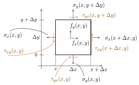
The stresses cannot be arbitrary functions of position. Equilibrium of a small block of material relates their derivatives to the body force. Consider the element in Figure 8.7.5, of size \(\Delta x\) by \(\Delta y\), loaded by a body force per unit volume \(\bm f\).
Figure 8.7.5: Stresses on the faces of an infinitesimal element.
Summing forces in the \(x\) direction, each stress is multiplied by the area of the face it acts on, and the body force by the volume of the element,
\[
\sum F_x = 0: \quad
\Delta\sigma_x\, \Delta y + \Delta\tau_{yx}\, \Delta x + f_x\, \Delta x \Delta y = 0
\]
which written out in full reads
\[
\left(\sigma_x(x+\Delta x, y) - \sigma_x(x,y)\right)\Delta y
+ \left(\tau_{yx}(x, y+\Delta y) - \tau_{yx}(x,y)\right)\Delta x
+ f_x\,\Delta x \Delta y = 0
\]
Dividing by \(\Delta x \Delta y\) and letting the element shrink turns the differences into partial derivatives. Doing the same in the \(y\) direction gives the pair
which is the equilibrium equation of continuum mechanics. It is the direct descendant of \(\sum F_i = 0\) from statics, written for a body in which the internal force varies continuously from point to point. Every structural problem in this book is 8.7.8 together with a constitutive law and a set of boundary conditions, and the various beam and rod and truss theories are what 8.7.8 becomes once a particular geometry is assumed.
Symmetry of the stress tensor
Force equilibrium is not the only condition. Taking moments about the midpoint of the element, the shear stresses on opposite faces each contribute a couple,
\[
\tau_{xy}(x+\Delta x, y)\,\Delta y\,\tfrac{1}{2}\Delta x
+ \tau_{xy}(x,y)\,\Delta y\,\tfrac{1}{2}\Delta x
- \tau_{yx}(x,y+\Delta y)\,\Delta x\,\tfrac{1}{2}\Delta y
- \tau_{yx}(x,y)\,\Delta x\,\tfrac{1}{2}\Delta y = 0
\]
The factors \(\tfrac{1}{2}\Delta x \Delta y\) are common to all four terms and cancel, leaving
and in the limit \(\Delta x \to 0\), \(\Delta y \to 0\) both sides become twice the value at the point, so \(\tau_{xy} = \tau_{yx}\). The same argument about the other two axes gives \(\tau_{yz} = \tau_{zy}\) and \(\tau_{xz} = \tau_{zx}\). The stress tensor is symmetric, and of its nine components only six are independent. Symmetry is what lets us diagonalise it later, and it is the reason the strain tensor was constructed symmetric to match.
Boundary traction
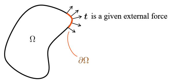
Equilibrium governs the interior. At the surface, the stress in the material must balance whatever is applied from outside. Let \(\Omega\) denote the body and \(\partial\Omega\) its boundary, and let an external force \(\bm t\) act on part of that boundary. This force is a traction, measured in force per unit length in two dimensions and force per unit area in three.
Figure 8.7.6: A traction applied to the boundary of a body.
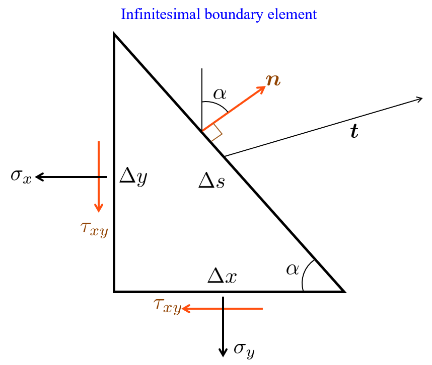
Cut a small triangular wedge from the boundary, as in Figure 8.7.7, with the traction acting on the hypotenuse of length \(\Delta s\) and the two straight legs lying along the coordinate directions. The leg with outward normal \(-\bm e_x\) has length \(\Delta y\) and the leg with outward normal \(-\bm e_y\) has length \(\Delta x\), and the outward unit normal of the hypotenuse has components
\[
\boxed{\bm\sigma \cdot \bm n = \bm t}
\tag{8.7.9}\]
The tensor is now doing exactly the job we asked of it at the start of the chapter. Feed it any direction \(\bm n\) and it returns the traction acting across a cut with that normal. The stress at a point is not a number and not even a list of three numbers, it is the linear map that turns cut directions into tractions.
A part of the boundary where the traction is prescribed, as a distributed load, a pressure \(\bm t = -p\,\bm n\) or a force, carries a Neumann boundary condition: through 8.7.9 it fixes the stress there, as \(EA\,du/dx(L) = F\) fixed the normal force at the end of the rod’s boundary value problem.
Example 1: Recovering the inclined cut
In Chapter 8.4 we computed the normal and shear stress on a cut inclined at an angle \(\varphi\) to the axis of a bar in uniaxial tension, and obtained 8.4.2 by writing equilibrium for that particular cut. Cauchy’s formula should reproduce the result without any new free body diagram, and it does.
A bar pulled along \(x\) with \(\sigma_0 = P/A\) has the stress tensor \(\bm\sigma = \operatorname{diag}(\sigma_0, 0)\): nothing acts in \(y\), and there is no shear in this frame. A cut at angle \(\varphi\) to the bar axis has unit normal \(\bm n = (\sin\varphi, -\cos\varphi)\) and unit tangent \(\bm m = (\cos\varphi, \sin\varphi)\). The traction on the cut is \(\bm t = \bm\sigma \bm n\), and its normal and tangential components are the projections of \(\bm t\) onto \(\bm n\) and \(\bm m\).
sigma_0, varphi = sp.symbols('sigma_0 varphi', real=True)sigma_uniaxial = sp.Matrix([[sigma_0, 0], [0, 0]])nn = sp.Matrix([sp.sin(varphi), -sp.cos(varphi)]) # normal of the cutmm = sp.Matrix([sp.cos(varphi), sp.sin(varphi)]) # tangent of the cuttt = sigma_uniaxial * nnsigma_phi = sp.simplify((tt.T * nn)[0])tau_phi = sp.simplify((tt.T * mm)[0])ltx(r"\bm t &=", tt,r"\\\sigma_\varphi &=", sigma_phi,r"\\\tau_\varphi &=", sp.simplify(sp.expand_trig(tau_phi)), aligned=True)
The results are \(\sigma_\varphi = \sigma_0\sin^2\varphi\) and \(\tau_\varphi = \sigma_0\sin\varphi\cos\varphi\), identical to 8.4.2 with \(\sigma_0 = P/A\). The earlier derivation needed a free body diagram for each new cut angle. The tensor needs none: one object encodes the response to every possible cut, and Cauchy’s formula extracts the answer for whichever cut we ask about.
Principal stress and strain
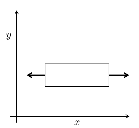
Consider a plate in pure tension along \(x\), as in Figure 8.7.8. Aligned with the load, the stress tensor is diagonal, with a normal stress along the load, some transverse component, and no shear at all.
Figure 8.7.8: Frame aligned with the load
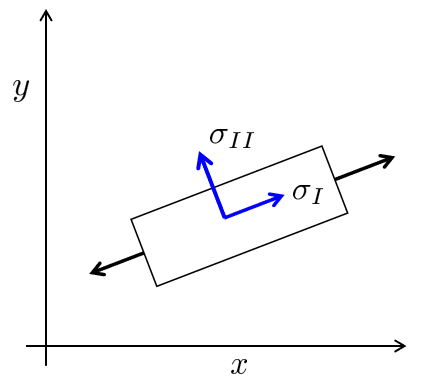
Figure 8.7.9: Frame rotated relative to the load
Rotate the frame of reference without touching the plate or the load, and shear stresses appear, exactly as they did in Example 1. Nothing physical changed, only our description of it. Reversing the question gives something useful: given a stress tensor with shear in it, is there a rotation that removes the shear entirely? The directions in which it vanishes are the principal directions, and the normal stresses in those directions are the principal stresses.
Figure 8.7.10: Rotating the frame changes the components while the state stays the same.
The shear on a cut vanishes when the traction is parallel to the normal, that is when
\[
\bm t = \lambda \bm n
\]
for some scalar \(\lambda\). Substituting Cauchy’s formula 8.7.9 gives
\[
\bm\sigma \cdot \bm n = \lambda \bm n
\quad\Longleftrightarrow\quad
(\bm\sigma - \lambda \bm I)\cdot \bm n = \bm 0
\tag{8.7.10}\]
which is an eigenvalue problem. The principal stresses are the eigenvalues of the stress tensor and the principal directions are its eigenvectors. Because the tensor is symmetric, the eigenvalues are real and the eigenvectors are mutually orthogonal, so the principal directions always form a proper coordinate frame.
Non-trivial solutions require the matrix to be singular, \(\det(\bm\sigma - \lambda\bm I) = 0\), which in two dimensions expands to
whose roots are the two principal stresses. The coefficients are the trace and the determinant, both of which are unchanged by rotation, which is the algebraic statement of the physical fact that the principal stresses do not depend on the frame we happened to start in. Solving the quadratic gives the closed form
half the difference between the largest and the smallest of the three principal stresses. Under uniaxial tension \(\sigma_0\) the principal stresses are \(\sigma_0\), \(0\) and \(0\), so \(\tau_{\max} = \sigma_0/2\) acts on the planes at \(45^\circ\) to the load, as 8.4.2 found by cutting. Mohr’s circle draws the two in-plane principal stresses as the points where a circle crosses the \(\sigma\) axis and the largest in-plane shear stress as its radius, and shows how they move as the frame turns.
Let us confirm 8.7.12 by solving the eigenvalue problem symbolically.
In three dimensions the stress tensor 8.7.6 is a \(3\times 3\) matrix, and the condition \(\det(\bm\sigma - \lambda\bm I) = 0\) is a cubic in \(\lambda\). Expanding the determinant and collecting powers of \(\lambda\) gives \(\det(\bm\sigma - \lambda\bm I) = -\lambda^3 + I_1\lambda^2 - I_2\lambda + I_3\), so the principal stresses are the three roots of the characteristic equation
They play the part that the trace and the determinant played in 8.7.11. Turning the frame by an orthogonal matrix \(\bm Q\), with \(\bm Q^\mathsf{T}\bm Q = \bm I\), changes the components to \(\bm\sigma' = \bm Q^\mathsf{T}\bm\sigma\bm Q\), the rule we met for the strain in Remark 8.7.1, and the characteristic polynomial does not notice,
since \(\det\bm Q^\mathsf{T}\det\bm Q = \det(\bm Q^\mathsf{T}\bm Q) = 1\). The polynomial is the same in every frame, and so are its coefficients and its roots. The six components describe the stress state together with our choice of axes; \(I_1\), \(I_2\) and \(I_3\) describe the state alone, and so does any quantity built from them, the von Mises stress below among them. In the principal frame the tensor is diagonal and the invariants read
which gives a check on any set of principal stresses we compute. SymPy confirms the expansion 8.7.15, and shows what becomes of the cubic in plane stress, \(\sigma_z = \tau_{xz} = \tau_{yz} = 0\).
The sum vanishes for every stress state. In plane stress \(I_3 = 0\) and the cubic factors into \(\lambda\) times the quadratic of 8.7.11: one principal stress is zero and the other two are the roots of the two-dimensional problem.
A symmetric tensor has three real roots, and we name them by size,
so that \(\sigma_1\) is the largest principal stress, the most tensile, \(\sigma_3\) the smallest, the most compressive, and \(\sigma_2\) the intermediate principal stress. The order counts the sign. A state with principal stresses \(-20\), \(-80\) and \(-150~\text{MPa}\) has \(\sigma_1 = -20~\text{MPa}\), the least compressive of the three. The principal directions \(\bm n_1\), \(\bm n_2\) and \(\bm n_3\) take the numbers of their principal stresses, and the principal strains are named the same way, \(\varepsilon_1 \ge \varepsilon_2 \ge \varepsilon_3\). In this notation 8.7.14 reads
\[
\tau_{\max} = \frac{\sigma_1 - \sigma_3}{2}
\]
and the intermediate principal stress does not enter it.
When the two shear stresses that involve \(z\) vanish, \(\tau_{xz} = \tau_{yz} = 0\), Cauchy’s formula gives \(\bm\sigma\bm e_z = \sigma_z\bm e_z\), so \(\bm e_z\) is a principal direction with the principal stress \(\sigma_z\). The determinant splits into \((\sigma_z - \lambda)\left[(\sigma_x - \lambda)(\sigma_y - \lambda) - \tau_{xy}^2\right]\), and the other two principal stresses follow from 8.7.12, with their directions in the \(xy\) plane. Which number \(\sigma_z\) receives depends on where it falls relative to that pair.
Plane stress is the case \(\sigma_z = 0\). In a two-dimensional problem the two roots of 8.7.12 are all the principal stresses there are, and calling them \(\sigma_1 \ge \sigma_2\) follows the same convention. A plate in plane stress is a three-dimensional body, however, with a third principal stress of zero normal to its surface. We therefore call the two roots the in-plane principal stresses and write them \(\sigma_\text{I} \ge \sigma_\text{II}\), keeping the Arabic numbers for the ordered three. The zero takes its place among them according to the signs of the in-plane pair:
Only in the second case is the largest in-plane shear stress, \((\sigma_\text{I} - \sigma_\text{II})/2\), also the largest over all planes. In the first case the maximum is \(\sigma_\text{I}/2\), on planes inclined at \(45^\circ\) to the surface of the plate, and in the third it is \(-\sigma_\text{II}/2\).
With all three shear stresses non-zero nothing splits off, and the cubic has to be solved as it stands. Cardano’s formula gives its roots in closed form, but in practice they are computed numerically, as the eigenvalues of a symmetric matrix. The NumPy function numpy.linalg.eigh returns them in ascending order together with orthonormal eigenvectors, and reversing that order gives 8.7.20. The normal and shear stress on every cut through the point lie in the region between three circles, one through each pair of principal stresses, as the section on three dimensions of the Mohr’s circle chapter shows. Example 3 does this for a full three-dimensional state.
Effective stress and the von Mises criterion
A design check needs a single number to compare against the yield strength, and a stress state has six components. Reducing them to one number requires a hypothesis about what causes yielding. The hypothesis that works best for ductile metals is that yielding is driven by distortion rather than by volume change, which is the von Mises criterion. In terms of the three principal stresses it reads
The two expressions give the same number, since 8.7.21 is written in the principal frame where the shear terms vanish. Note that adding the same pressure to all three normal stresses leaves \(\sigma_{\text{vM}}\) unchanged, because only differences of principal stresses appear. Hydrostatic pressure does not cause yielding, which is why material deep in the ocean does not yield under its own ambient pressure.
For plane stress, where \(\sigma_z = \tau_{yz} = \tau_{zx} = 0\), 8.7.22 simplifies to
which is the form that appears in most hand calculations, and the quantity that a finite element post-processor plots by default. Chapter 8.10 derives the criterion from the distortion energy and compares it with the Tresca and maximum normal stress criteria.
Example 2: Evaluating a plane stress state
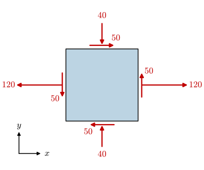
A point in a loaded plate is in the plane stress state \(\sigma_x = 120~\text{MPa}\), \(\sigma_y = -40~\text{MPa}\), \(\tau_{xy} = 50~\text{MPa}\), Figure 8.7.11. Determine the principal stresses, the principal directions, the maximum shear stress and the von Mises stress. The material yields at \(250~\text{MPa}\): is the point safe?
Figure 8.7.11: The plane stress element of Example 2, with the stresses in MPa. Each arrow is drawn the way its stress acts, so the arrows of the compressive \(\sigma_y = -40~\text{MPa}\) point into the element.
The normal \(\bm e_z\) of the plate carries no stress, so it is a principal direction with principal stress zero. The in-plane principal stresses follow from 8.7.12,
and the direction \(\bm n_\text{I} = (\cos\theta_\text{I}, \sin\theta_\text{I})\) from the first row of \((\bm\sigma - \sigma_\text{I}\bm I)\bm n_\text{I} = \bm 0\), 8.7.10,
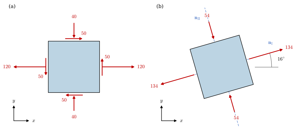
Figure 8.7.12 draws the result onto the element of Figure 8.7.11. Turned by \(\theta_\text{I}\), the element carries only the two principal stresses: tension along \(\bm n_\text{I}\) and compression along \(\bm n_\text{II}\), and no shear on any of its faces.
Code
from matplotlib.patches import FancyArrowPatch, Polygonfrom mechanicskit import sketch as skdef arrow(ax, p0, p1, color=sk.LOAD, lw=1.8): ax.add_patch(FancyArrowPatch(p0, p1, arrowstyle='-|>', mutation_scale=12, color=color, lw=lw, shrinkA=0, shrinkB=0, zorder=6))def element(ax, theta, normal, shear, h=1.0, k=1/120, g=0.12):"""A square of half side h turned by theta, with a normal stress on each pair of faces (normal[0] on the faces along e1, normal[1] on those along e2) and the shear on all four.""" c, s = np.cos(theta), np.sin(theta) e1, e2 = np.array([c, s]), np.array([-s, c]) ax.add_patch(Polygon([h*(-e1 - e2), h*(e1 - e2), h*(e1 + e2), h*(-e1 + e2)], closed=True, facecolor=sk.STEEL, edgecolor=sk.EDGE, lw=sk.LW, zorder=2))for n, sig in ((e1, normal[0]), (-e1, normal[0]), (e2, normal[1]), (-e2, normal[1])): L =0.25+ k*abs(sig) face = (h + g)*n# tension leaves the face, compression points into it arrow(ax, *((face, face + L*n) if sig >0else (face + L*n, face))) sk.label(ax, face + (L +0.25)*n, f'${abs(sig):.0f}$', color=sk.LOAD, fontsize=12)if shear !=0: Ls =0.25+ k*abs(shear)for n, t in ((e1, e2), (-e1, -e2), (e2, e1), (-e2, -e1)): mid = (h +0.1)*n arrow(ax, mid - Ls/2*t, mid + Ls/2*t) sk.label(ax, mid + (Ls/2+0.05)*t +0.2*n, f'${abs(shear):.0f}$', color=sk.LOAD, fontsize=12)return e1, e2th =float(sp.rad(theta_I))fig, (ax, bx) = plt.subplots(1, 2, figsize=(10, 4.8))for a in (ax, bx): a.set_aspect('equal') a.axis('off') a.set_xlim(-2.7, 2.7) a.set_ylim(-2.5, 2.5)# the given state, as in the problem statementelement(ax, 0.0, (120, -40), 50)# the principal state: sigma_I along n_I, sigma_II along n_II, no sheare1, e2 = element(bx, th, (float(sigma_I), float(sigma_II)), 0)for a in (ax, bx): # the frame at the lower left o = np.array([-2.35, -2.1])for d, name in (((1, 0), '$x$'), ((0, 1), '$y$')): arrow(a, o, o +0.6*np.array(d), color=sk.EDGE, lw=1.2) sk.label(a, o +0.78*np.array(d), name, fontsize=12)# the principal directions through the centre, and the angle from the x axisfor d, name, side in ((e1, r'$\mathbf{n}_\mathrm{I}$', e2), (e2, r'$\mathbf{n}_\mathrm{II}$', -e1)): bx.plot(*np.c_[-2.4*d, 2.4*d], color=sk.BLUE, lw=0.9, ls=(0, (6, 3)), zorder=1) sk.label(bx, 2.1*d +0.38*side, name, color=sk.BLUE, fontsize=12)# the angle from the x direction to n_I, drawn outside the elementr0, r1, ra =1.3, 2.2, 1.95bx.plot([r0, r1], [0, 0], color=sk.GREY, lw=0.9, zorder=3)t = np.linspace(0, th, 30)bx.plot(ra*np.cos(t), ra*np.sin(t), color=sk.GREY, lw=0.9, zorder=3)sk.label(bx, (ra +0.35)*np.array([np.cos(th/2), np.sin(th/2)]) + np.array([0.05, -0.02]),rf'${float(theta_I):.0f}^{{\circ}}$', fontsize=12)sk.label(ax, (-2.55, 2.35), '(a)', fontsize=12, ha='left')sk.label(bx, (-2.55, 2.35), '(b)', fontsize=12, ha='left')fig.tight_layout()plt.show()
Figure 8.7.12: The element of Example 2 with the stresses in MPa. (a) The given state in the \(x\), \(y\) frame, as in Figure 8.7.11. (b) The same state on an element turned by \(\theta_\text{I} = 16^\circ\): the tension \(\sigma_\text{I} = 134~\text{MPa}\) acts along \(\bm n_\text{I}\) and the compression \(\sigma_\text{II} = -54~\text{MPa}\) along \(\bm n_\text{II}\), and the faces carry no shear.
The in-plane principal stresses are \(\sigma_\text{I} = 134~\text{MPa}\) in tension and \(\sigma_\text{II} = -54~\text{MPa}\) in compression. The direction \(\bm n_\text{I}\) makes an angle of \(16^\circ\) with the \(x\) axis, which is the amount the frame must be rotated for the shear to disappear.
The pair has opposite signs, the second case of the plane stress ordering, so the zero normal to the plate falls between them and the ordered principal stresses 8.7.20 are
The maximum shear stress in the plane is half the difference of the in-plane pair, a result that follows from 8.4.2 applied to the principal frame, and the largest shear stress over all planes is 8.7.14,
The von Mises stress is \(168~\text{MPa}\) against a yield strength of \(250~\text{MPa}\), so the point is elastic with a factor of safety of \(1.49\). the chapter on Mohr’s circle draws this state as a circle, and its interactive figure loads it as a preset. The two shear values coincide here because the in-plane pair has opposite signs: the zero normal to the plate is \(\sigma_2\), and the pair itself already spans \(\sigma_1\) and \(\sigma_3\). Had both in-plane principal stresses been positive, the zero would have been \(\sigma_3\), the absolute maximum would have been \(\sigma_\text{I}/2\), and the two numbers would differ. Observe also that the largest principal stress, \(\sigma_1 = 134~\text{MPa}\), is smaller than the effective stress. A check based on the largest normal stress alone would have reported a factor of safety of \(1.9\) and been optimistic by a quarter. Combined stress states have to be reduced through a failure criterion, not by picking the largest component.
Example 3: Principal stresses of a three-dimensional state
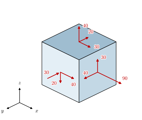
A finite element model of a forged steel part reports, at a point in its interior, the stress components
shown in Figure 8.7.13. Determine the principal stresses \(\sigma_1 \ge \sigma_2 \ge \sigma_3\) and their directions, the maximum shear stress and the von Mises stress.
Figure 8.7.13: The stress components of Example 3 in MPa on the three visible faces of a cube at the point. Each arrow is drawn the way its stress acts, so the compressive \(\sigma_y\) points into its face and the two arrows of \(\tau_{yz} = -20~\text{MPa}\) point along \(-z\) on the \(y\) face and along \(-y\) on the \(z\) face. The hidden faces carry the same stresses in the opposite directions.
All three shear stresses are non-zero, so no principal direction can be read off and the full cubic 8.7.15 has to be solved. Its coefficients follow from 8.7.16, 8.7.17 and 8.7.18,
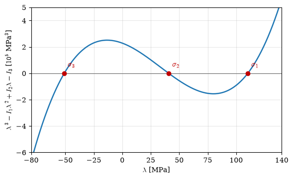
The roots are \(\sigma_1 = 110.2~\text{MPa}\), \(\sigma_2 = 40.8~\text{MPa}\) and \(\sigma_3 = -51.0~\text{MPa}\). One is compressive and two are tensile, and the intermediate one is far from zero, so that this state is not close to plane stress in any frame. Figure 8.7.14 shows the cubic crossing zero at the three roots.
Figure 8.7.14: The characteristic polynomial of Example 3 against \(\lambda\). Its three zeros are the principal stresses, numbered from the right by 8.7.20.
The principal directions are the eigenvectors of 8.7.10. We collect them as the columns of the matrix \(\bm N = [\bm n_1\;\bm n_2\;\bm n_3]\), which numpy.linalg.eigh returns, with the eigenvalues, in ascending order; reversing the columns puts them in the order of 8.7.20. In the principal frame the tensor is diagonal,
and the directions are orthonormal, \(\bm N^\mathsf{T}\bm N = \bm I\). The eigenvalues must also agree with the roots of the cubic and reproduce the invariants by 8.7.19.
Code
Sigma_ex = np.array([[s_x, t_xy, t_xz], [t_xy, s_y, t_yz], [t_xz, t_yz, s_z]], dtype=float)w, V = np.linalg.eigh(Sigma_ex) # ascending eigenvalues, orthonormal columnsw, N = w[::-1], V[:, ::-1] # reversed: sigma_1 >= sigma_2 >= sigma_3s1, s2, s3 = wltx(r"\bm N = [\bm n_1\;\bm n_2\;\bm n_3] &=", N,r"\\\bm N^\mathsf{T}\bm\sigma\bm N &=", np.round(N.T @ Sigma_ex @ N, 9) +0.0,r"~\text{MPa}, \qquad \bm N^\mathsf{T}\bm N =", np.round(N.T @ N, 12) +0.0, aligned=True, precision=4)
The eigenvalues agree with the roots to round-off, and the three invariants are reproduced. The first column of \(\bm N\) is the direction of the largest tensile stress, \(\bm n_1 \approx (0.92, 0.22, 0.33)\) up to sign, close to \(x\) and tipped toward \(z\), where \(\sigma_x\) and \(\sigma_z\) are the two largest normal components and \(\tau_{xz}\) couples them.
The maximum shear stress is 8.7.14, and the von Mises stress is 8.7.21,
The largest shear stress is \(80.6~\text{MPa}\), on the planes that bisect the angle between \(\bm n_1\) and \(\bm n_3\), and the von Mises stress is \(140~\text{MPa}\) by both routes. The intermediate principal stress \(\sigma_2 = 40.8~\text{MPa}\) does not enter \(\tau_{\max}\) but does enter \(\sigma_{\text{vM}}\), and on this point the two yield criteria of Chapter 8.10 part ways.
What comes next
We now have a complete kinematic description in 8.7.3, a complete equilibrium statement in 8.7.8, and a boundary condition in 8.7.9. What is missing is the link between stress and strain in more than one dimension. Hooke’s law \(\sigma = E\varepsilon\) relates one component to one component; the generalisation to tensors is the subject of Chapter 8.9, and with it in hand the continuum model is closed and can be specialised to any geometry we like.