Stability in a model with one degree of freedom

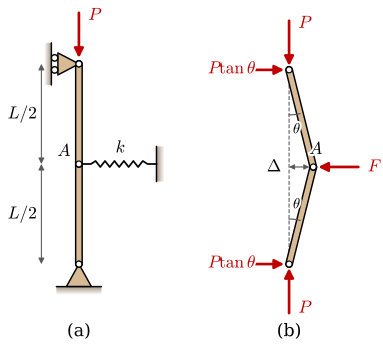
The mechanism is easiest to see in a model whose only flexibility is a spring, Figure 8.18.1. Two rigid bars of length \(L/2\) are pinned together at \(A\). The foot is pinned to the ground, the head is held in a slot that lets it move up and down but not sideways, and a spring of stiffness \(k\) holds \(A\) against sideways motion. A load \(P\) presses down on the head.

Suppose the joint is pushed sideways by \(\Delta = (L/2)\sin\theta\), panel (b). Each bar carries no load between its ends, so the force in it acts along it. At the head, the vertical reaction \(P\) and the horizontal reaction \(H\) therefore add up to a force along the tilted upper bar, and \(H/P = \tan\theta\). The same holds at the foot. Horizontal equilibrium of the whole model then requires the spring to deliver

\[ F = 2P\tan\theta \]

while the spring itself, stretched by \(\Delta\), delivers

\[ F = k\Delta = k\frac{L}{2}\sin\theta . \]

The two must agree for the displaced shape to be in equilibrium. For small angles, \(\sin\theta \approx \tan\theta \approx \theta\), and the comparison reduces to the restoring force \(kL\theta/2\) of the spring against the disturbing force \(2P\theta\) of the load. The angle cancels, so the outcome is decided by the load alone, and the two forces balance at the single load

\[ \boxed{P_{\text{cr}} = \frac{kL}{4}} \tag{8.18.1}\]

the critical load. It separates three cases:

• Stable equilibrium, \(P < P_{\text{cr}}\): the spring supplies more force than the load demands and pushes the joint back to the straight position.
• Neutral equilibrium, \(P = P_{\text{cr}}\): the displaced shape is in equilibrium for every small \(\theta\).
• Unstable equilibrium, \(P > P_{\text{cr}}\): the load demands more force than the spring can give, and any disturbance grows.

Without the small-angle approximation, equilibrium requires \(k(L/2)\sin\theta = 2P\tan\theta\), which either holds with \(\theta = 0\) for any load, or with

\[ \frac{P}{P_{\text{cr}}} = \cos\theta . \]

The total potential energy of the model gives the same result by a second route, and also decides the stability of each branch. It is the energy stored in the spring minus the work of the load, whose point of application has moved down by \(L(1 - \cos\theta)\),

\[ \Pi(\theta) = \frac{1}{2}k\left(\frac{L}{2}\sin\theta\right)^2 - PL(1 - \cos\theta) \]

Equilibrium requires \(d\Pi/d\theta = 0\), and the equilibrium is stable where \(d^2\Pi/d\theta^2 > 0\), so that the energy has a minimum there.

theta, k, L, P = sp.symbols('theta k L P', positive=True)

Pi = sp.Rational(1, 2)*k*(L/2*sp.sin(theta))**2 - P*L*(1 - sp.cos(theta))
dPi = sp.factor(sp.diff(Pi, theta))
d2Pi_straight = sp.diff(Pi, theta, 2).subs(theta, 0)
d2Pi_branch = sp.simplify(sp.diff(Pi, theta, 2).subs(P, k*L*sp.cos(theta)/4))

ltx(r"\frac{d\Pi}{d\theta} &=", dPi,
    r"\\ \frac{d^2\Pi}{d\theta^2}\Big|_{\theta = 0} &=", d2Pi_straight,
    r"\\ \frac{d^2\Pi}{d\theta^2}\Big|_{P = P_{\text{cr}}\cos\theta} &=", d2Pi_branch,
    aligned=True)

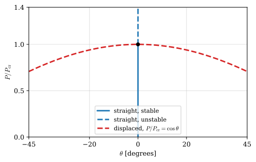
The first derivative vanishes for \(\sin\theta = 0\) or for \(P = (kL/4)\cos\theta\), the two branches found from equilibrium. On the straight branch the second derivative is positive for \(P < kL/4\) and negative above, confirming 8.18.1. On the displaced branch it is negative for every \(\theta \neq 0\), so the displaced equilibrium is unstable as well. Figure 8.18.2 draws both branches. Where they cross, at \(P = P_{\text{cr}}\), the solution bifurcates: the straight path continues but loses its stability, and a second path branches off.

th = np.radians(np.linspace(-45, 45, 200))

fig, ax = plt.subplots(figsize=(6, 3.6))
ax.plot([0, 0], [0, 1], color='C0', lw=2.2, label='straight, stable')
ax.plot([0, 0], [1, 1.4], color='C0', lw=2.2, ls='--', label='straight, unstable')
ax.plot(np.degrees(th), np.cos(th), color='C3', lw=2.2, ls='--',
        label=r'displaced, $P/P_{\mathrm{cr}} = \cos\theta$')
ax.plot(0, 1, 'o', color='black', ms=5)
ax.set_xlabel(r'$\theta$ [degrees]')
ax.set_ylabel(r'$P/P_{\mathrm{cr}}$')
ax.set_xticks([-45, -20, 0, 20, 45])
ax.set_yticks([0, 0.5, 1, 1.4])
ax.set_xlim(-45, 45)
ax.set_ylim(0, 1.4)
ax.grid(True, alpha=0.4)
ax.legend(loc='lower center', fontsize=9)
plt.show()

A real model is never perfectly straight, and an imperfect one does not reach the bifurcation point. It starts to deflect from the first increment of load, and in this model it collapses at a load below \(P_{\text{cr}}\), since the displaced branch falls away on both sides. The continuous column of the next section behaves more kindly: its buckled branch rises very slightly, so it goes on carrying the critical load while it deflects. Either way, \(P_{\text{cr}}\) is the load at which the structure loses its stiffness against the buckling shape, and it is the number design starts from.

The pinned column and Euler’s critical load

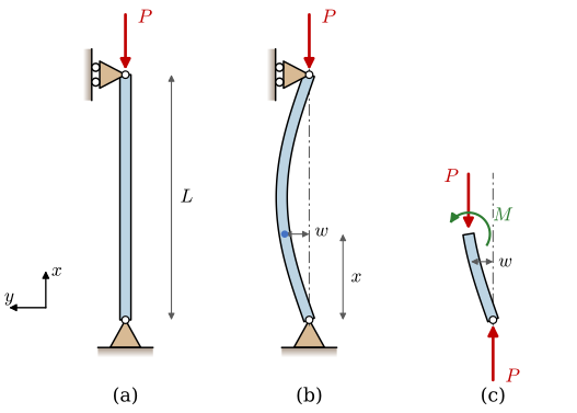
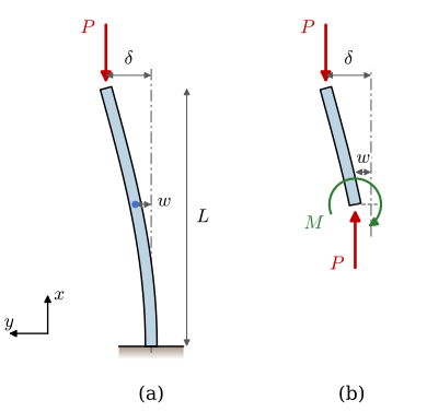
We replace the rigid bars and the spring by an elastic column, Figure 8.18.3. The ideal column is perfectly straight, made of a homogeneous linear elastic material, and loaded exactly through the centroids of its end sections, so that without a disturbance it only shortens. Both ends are pinned, the head being free to move along the axis. Its deflections are small, and it bends according to the Euler-Bernoulli theory of Chapter 8.16. We take \(x\) along the column from its foot and \(y\) across it, as in the beam chapter turned a quarter turn anticlockwise, so that \(w\) is positive to the left in the figure.

The spring of the model is now the bending stiffness of the column itself, with no hinge and no spring to point at, and the question is where the restoring moment comes from. The answer is the moment-curvature relation 8.16.9, \(M = EIw''\): a bent column resists with a moment proportional to its curvature. The disturbing moment comes from equilibrium of the free body in panel (c), and here lies the one new step. The moment is taken about the cut in the deformed position, where the reaction \(P\) at the foot has the lever arm \(w\),

\[ M + Pw = 0 . \]

With 8.16.9 this gives the differential equation of the buckled column,

\[ EI\frac{d^2w}{dx^2} = -Pw \qquad\text{or}\qquad \frac{d^2w}{dx^2} + \alpha^2 w = 0, \quad \alpha^2 = \frac{P}{EI} \tag{8.18.2}\]

The general solution is \(w = C_1\sin\alpha x + C_2\cos\alpha x\), and the pins prescribe \(w(0) = 0\) and \(w(L) = 0\). Written as a linear system for the two constants,

\[ \begin{bmatrix} 0 & 1 \\ \sin\alpha L & \cos\alpha L \end{bmatrix} \begin{bmatrix} C_1 \\ C_2 \end{bmatrix} = \begin{bmatrix} 0 \\ 0 \end{bmatrix} \]

the system is homogeneous. It always has the solution \(C_1 = C_2 = 0\), the straight column, which is an equilibrium at any load. A deflected equilibrium exists only when the determinant vanishes, and that is a condition on the load.

x, alpha, EI = sp.symbols('x alpha EI', positive=True)
C1, C2 = sp.symbols('C_1 C_2', real=True)

w = C1*sp.sin(alpha*x) + C2*sp.cos(alpha*x)
residual = sp.simplify(sp.diff(w, x, 2) + alpha**2*w)          # @eq-column-pinned

conditions = [w.subs(x, 0), w.subs(x, L)]                       # pinned at both ends
A_bc = sp.Matrix([[sp.diff(c, Ci) for Ci in (C1, C2)] for c in conditions])

ltx(r"w'' + \alpha^2 w =", residual, r",\qquad \det\begin{bmatrix} 0 & 1 \\ \sin\alpha L & \cos\alpha L \end{bmatrix} =",
    A_bc.det())

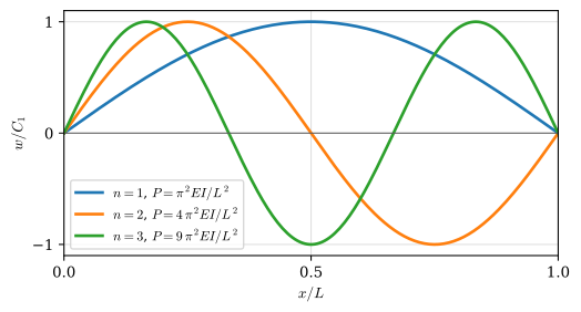
The determinant vanishes when \(\sin\alpha L = 0\), that is for \(\alpha L = n\pi\) with \(n = 1, 2, 3, \ldots\) Then \(C_2 = 0\) while \(C_1\) is left free, and the column has the deflected equilibrium shapes \(w = C_1\sin(n\pi x/L)\) at the loads \(P = n^2\pi^2 EI/L^2\). The smallest, \(n = 1\), is the load at which a pinned column buckles,

\[ \boxed{P_{\text{cr}} = \frac{\pi^2 EI}{L^2}} \tag{8.18.3}\]

Euler’s critical load. Leonhard Euler found it while studying elastic curves in 1744 and treated the column on its own in a memoir read to the Berlin Academy in 1757 [1]. The problem is an eigenvalue problem: the differential equation and its boundary conditions have non-zero solutions only for particular values of the parameter \(\alpha\), and the solutions themselves, the buckling modes of Figure 8.18.4, are known only up to the amplitude \(C_1\). The amplitude stays free for the same reason as the angle \(\theta\) of the spring model: at the critical load every small deflection of the buckled shape is an equilibrium, so the small-deflection theory tells at which load and in which shape the column buckles, but not how far.

s = np.linspace(0, 1, 200)

fig, ax = plt.subplots(figsize=(6, 3.0))
for n, c in zip((1, 2, 3), ('C0', 'C1', 'C2')):
    factor = '' if n == 1 else rf'{n**2}\,'
    ax.plot(s, np.sin(n*np.pi*s), color=c, lw=2,
            label=rf'$n = {n}$, $P = {factor}\pi^2 EI/L^2$')
ax.axhline(0, color='0.35', lw=0.8)
ax.set_xlabel('$x/L$')
ax.set_ylabel('$w/C_1$')
ax.set_xticks([0, 0.5, 1])
ax.set_yticks([-1, 0, 1])
ax.set_xlim(0, 1)
ax.grid(True, alpha=0.4)
ax.legend(fontsize=9, loc='lower left')
plt.show()

A column braced sideways at its midpoint cannot buckle in the first mode, since the brace holds the point where that mode has its largest deflection. It buckles in the second mode instead, which has a node at the brace, at four times the load. Bracing a long column at a few points is the cheapest way to raise its critical load.

Two consequences of 8.18.3 shape every column design. The material enters only through \(E\): a high-strength steel buckles at the same load as a mild steel with the same modulus. And the length enters squared, so a column twice as long carries a quarter of the load. The truss notebook of the bridge lab, mechanics.ju.se/marimo/trussAnalysis, uses 8.18.3 in this way. A truss bar is pinned at both ends and carries only an axial force, so the notebook checks every compressed bar against its own Euler load \(\pi^2 EI/L^2\), and a long compressed bar may need a thicker profile than its stress alone would ask for.

Critical stress and slenderness

Dividing the critical load by the cross-sectional area gives the average stress at which the column buckles. With the radius of gyration \(r = \sqrt{I/A}\), the second moment of area becomes \(I = Ar^2\), and

\[ \sigma_{\text{cr}} = \frac{P_{\text{cr}}}{A} = \frac{\pi^2 E A r^2}{A L^2} = \frac{\pi^2 E}{(L/r)^2} = \frac{\pi^2 E}{\lambda^2} \tag{8.18.4}\]

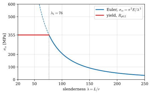
The ratio \(\lambda = L/r\) is the slenderness ratio, the single geometric number that decides how easily a column buckles. Swedish texts often write \(i\) for the radius of gyration [2]. Figure 8.18.5 plots 8.18.4 for steel. Euler’s formula assumes a linear elastic material, so it holds only where it predicts a stress below the proportional limit, which for steel lies close to the yield strength \(R_{p0.2}\). The two curves meet at the slenderness

\[ \lambda_1 = \pi\sqrt{\frac{E}{R_{p0.2}}} \]

and columns more slender than that buckle elastically, while stockier columns yield before Euler’s load is reached.

E_steel, R_p = 210e3, 355                       # MPa, a structural steel S355
lam = np.linspace(20, 250, 300)
lam_1 = np.pi*np.sqrt(E_steel/R_p)
sigma_cr = np.pi**2*E_steel/lam**2              # @eq-euler-stress

fig, ax = plt.subplots(figsize=(6, 3.6))
ax.plot(lam, sigma_cr, color='C0', lw=1.2, ls='--')
ax.plot(lam[lam >= lam_1], sigma_cr[lam >= lam_1], color='C0', lw=2.2,
        label=r'Euler, $\sigma_{\mathrm{cr}} = \pi^2 E/\lambda^2$')
ax.plot([20, lam_1], [R_p, R_p], color='C3', lw=2.2, label=r'yield, $R_{p0.2}$')
ax.axvline(lam_1, color='0.35', lw=0.8, ls=':')
ax.text(lam_1 + 3, 520, rf'$\lambda_1 = {lam_1:.0f}$', fontsize=10)
ax.set_xlabel(r'slenderness $\lambda = L/r$')
ax.set_ylabel(r'$\sigma_{\mathrm{cr}}$ [MPa]')
ax.set_xticks([20, 50, 100, 150, 200, 250])
ax.set_yticks([0, 100, 200, 355, 500, 600])
ax.set_xlim(20, 250)
ax.set_ylim(0, 600)
ax.grid(True, alpha=0.4)
ax.legend()
plt.show()

Other end conditions and the effective length

The column of Figure 8.18.6 is clamped at its foot and free at its head, like a flagpole or a post loaded from above. The load stays vertical as the head moves sideways by \(\delta\). Equilibrium of the part above a cut at \(x\), panel (b), taken again about the cut in the deformed position, gives the moment

\[ M = P(\delta - w) \]

and with 8.16.9 the differential equation

\[ \frac{d^2w}{dx^2} + \alpha^2 w = \alpha^2\delta \]

whose general solution is \(w = C_1\sin\alpha x + C_2\cos\alpha x + \delta\). The clamp prescribes \(w(0) = 0\) and \(w'(0) = 0\), which give \(C_2 = -\delta\) and \(C_1 = 0\). The deflection at the head must equal \(\delta\), which closes the problem.

delta = sp.symbols('delta', positive=True)
wf = sp.Function('w')

sol = sp.dsolve(sp.Eq(wf(x).diff(x, 2) + alpha**2*wf(x), alpha**2*delta), wf(x),
                ics={wf(0): 0, wf(x).diff(x).subs(x, 0): 0}).rhs
head = sp.simplify(sol.subs(x, L) - delta)

ltx(r"w(x) &=", sp.factor(sol), r"\\ w(L) - \delta &=", head, aligned=True)

A non-zero \(\delta\) requires \(\cos\alpha L = 0\), of which the smallest root is \(\alpha L = \pi/2\), so

\[ P_{\text{cr}} = \frac{\pi^2 EI}{4L^2} = \frac{\pi^2 EI}{(2L)^2} \]

a quarter of the load of a pinned column of the same length. The buckled shape \(w = \delta(1 - \cos\alpha x)\) is a quarter of a cosine wave, and mirrored about the head it is exactly the half sine wave of a pinned column of length \(2L\). Every end condition can be compared with the pinned column in this way, by writing

\[ \boxed{P_{\text{cr}} = \frac{\pi^2 EI}{L_e^2}, \qquad L_e = \beta L} \tag{8.18.5}\]

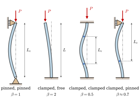
where the effective length \(L_e\) is the length of the equivalent pinned column, the distance between two points of inflection of the buckling mode. Figure 8.18.7 shows the four standard cases.

For the clamped-pinned column no free body gives the moment directly, because the clamp moment is unknown and the column is statically indeterminate. We then return to the slice equilibrium of 8.16.12 and write it, as for the free bodies above, on the deformed slice. The axial force \(N = -P\) acts on the two faces of the slice, which are offset sideways by \(dw\), and it adds the moment \(P\,dw\) to the moment balance. With no transverse load, \(dT/dx = 0\), and

\[ \frac{dM}{dx} = T - P\frac{dw}{dx} \qquad\Rightarrow\qquad EI\frac{d^4 w}{dx^4} + P\frac{d^2 w}{dx^2} = 0 \tag{8.18.6}\]

after differentiating once more and inserting 8.16.9. This fourth-order equation replaces the elastic line equation 8.16.13 for a beam under an axial compression. Its general solution has four constants,

\[ w = C_1\sin\alpha x + C_2\cos\alpha x + C_3 x + C_4 \]

and each end supplies two of the four boundary conditions. A clamped end has \(w = 0\) and \(w' = 0\), a pinned end \(w = 0\) and \(M = EIw'' = 0\). A free end has \(M = 0\) and no transverse force, and since \(T\) is now the force across the undeformed axis, that condition reads \(T = EI\,d^3w/dx^3 + P\,dw/dx = 0\). The four conditions form a homogeneous linear system for \(C_1, \ldots, C_4\), and as for the pinned column the critical load is the smallest \(\alpha\) that makes its determinant vanish. The code below sets up the system for each case and finds that root numerically, which gives \(\beta = \pi/(\alpha L)\).

C = sp.symbols('C_1:5', real=True)
w4 = C[0]*sp.sin(alpha*x) + C[1]*sp.cos(alpha*x) + C[2]*x + C[3]
d = lambda n, x0: sp.diff(w4, x, n).subs(x, x0)

# the two conditions of each end, divided by EI; P = alpha^2 EI
ends = {
    'clamped': lambda x0: [d(0, x0), d(1, x0)],
    'pinned':  lambda x0: [d(0, x0), d(2, x0)],
    'free':    lambda x0: [d(2, x0), d(3, x0) + alpha**2*d(1, x0)],
}

def beta(foot, head):
    """pi over the smallest alpha L at which the boundary-condition matrix is singular."""
    eqs = ends[foot](0) + ends[head](1)                         # L = 1
    det = sp.lambdify(alpha, sp.Matrix([[sp.diff(e, c) for c in C] for e in eqs]).det())
    a = np.linspace(0.5, 10, 2000)
    f = det(a)
    i = np.flatnonzero(np.sign(f[:-1]) != np.sign(f[1:]))[0]   # the first change of sign
    return np.pi/brentq(det, a[i], a[i + 1])

ltx(r"\beta_{\text{pinned, pinned}} &=", beta('pinned', 'pinned'),
    r"\\ \beta_{\text{clamped, free}} &=", beta('clamped', 'free'),
    r"\\ \beta_{\text{clamped, clamped}} &=", beta('clamped', 'clamped'),
    r"\\ \beta_{\text{clamped, pinned}} &=", beta('clamped', 'pinned'),
    aligned=True, precision=3)

The first two reproduce the closed-form results, and the clamped-clamped column, whose mode is a full cosine wave with inflection points at \(L/4\) and \(3L/4\), has \(\beta = 1/2\). The clamped-pinned column satisfies \(\tan\alpha L = \alpha L\), whose smallest root \(\alpha L = 4.493\) gives \(\beta = 0.699\), usually rounded to \(0.7\). The clamped-clamped column carries four times the load of the pinned one, and the clamped-free column a quarter of it, a factor of sixteen between the stiffest and the weakest support of the same column.

Eccentric load and the secant formula

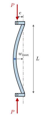
No real load passes exactly through the centroid. In Figure 8.18.8 the load acts at the eccentricity \(e\) from the axis at both ends of a pinned column. The column now bends from the first increment of load, and the question is no longer when a deflected shape becomes possible but how large the deflection and the stress become.

The load has the lever arm \(e + w\) about a cut at \(x\), so \(M = -P(e + w)\), and the differential equation becomes

\[ \frac{d^2w}{dx^2} + \alpha^2 w = -\alpha^2 e \]

with \(w(0) = w(L) = 0\). It is no longer homogeneous, and it has a unique solution for every load below the critical one.

e = sp.symbols('e', positive=True)

w_ecc = sp.dsolve(sp.Eq(wf(x).diff(x, 2) + alpha**2*wf(x), -alpha**2*e), wf(x),
                  ics={wf(0): 0, wf(L): 0}).rhs
w_mid = w_ecc.subs(x, L/2)
check = sp.simplify(w_mid - e*(1/sp.cos(alpha*L/2) - 1))

ltx(r"w(x) &=", sp.simplify(w_ecc), r"\\ w\left(\tfrac{L}{2}\right) - e\left(\sec\tfrac{\alpha L}{2} - 1\right) &=", check,
    aligned=True)

The largest deflection is therefore

\[ w_{\max} = e\left(\sec\frac{\alpha L}{2} - 1\right), \qquad \frac{\alpha L}{2} = \frac{\pi}{2}\sqrt{\frac{P}{P_{\text{cr}}}} \tag{8.18.7}\]

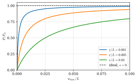
which grows without bound as \(P \to P_{\text{cr}}\), since the secant does as its argument approaches \(\pi/2\). Figure 8.18.9 plots the load against the deflection. A smaller eccentricity delays the bending but does not change where it ends: every curve approaches the critical load, and the ideal column is the limit \(e \to 0\), which stays straight up to \(P_{\text{cr}}\) and then deflects at constant load.

p = np.linspace(0, 0.995, 400)                       # P/P_cr
amp = 1/np.cos(np.pi/2*np.sqrt(p)) - 1               # w_max/e, @eq-eccentric-deflection

fig, ax = plt.subplots(figsize=(6, 3.6))
for e_L, c in zip((0.001, 0.005, 0.02), ('C0', 'C1', 'C2')):
    ax.plot(e_L*amp, p, color=c, lw=2, label=rf'$e/L = {e_L}$')
ax.plot([0, 0, 0.1], [0, 1, 1], color='black', lw=1.2, ls='--', label=r'ideal, $e = 0$')
ax.set_xlabel(r'$w_{\max}/L$')
ax.set_ylabel(r'$P/P_{\mathrm{cr}}$')
ax.set_xticks([0, 0.025, 0.05, 0.075, 0.1])
ax.set_yticks([0, 0.25, 0.5, 0.75, 1])
ax.set_xlim(0, 0.1)
ax.set_ylim(0, 1.05)
ax.grid(True, alpha=0.4)
ax.legend(loc='lower right')
plt.show()

The largest moment acts at mid-height, \(M_{\max} = P(e + w_{\max}) = Pe\sec(\alpha L/2)\). The largest compressive stress adds the bending stress 8.16.11 at the extreme fibre, at the distance \(c\) from the neutral axis, to the average stress \(P/A\). With \(I = Ar^2\) and \(\alpha L/2 = (L/2r)\sqrt{P/(EA)}\), this is the secant formula,

\[ \boxed{\sigma_{\max} = \frac{P}{A}\left[1 + \frac{ec}{r^2}\sec\left(\frac{L_e}{2r}\sqrt{\frac{P}{EA}}\right)\right]} \tag{8.18.8}\]

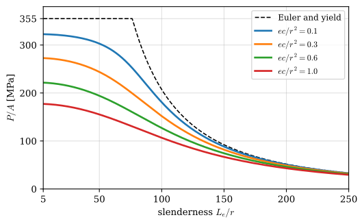
where the length \(L\) has been replaced by the effective length \(L_e\) to cover the other end conditions [3]. The dimensionless group \(ec/r^2\) is the eccentricity ratio. 8.18.8 is nonlinear in \(P\): doubling the load more than doubles the stress, and a factor of safety must be applied to the load, never to the stress. Solving it for the average stress \(P/A\) at which \(\sigma_{\max}\) reaches the yield strength gives the curves of Figure 8.18.10. For slender columns they approach Euler’s curve, and for stocky ones the yield strength reduced by the bending.

def secant_load(lam, ecr2, E=E_steel, sigma_y=R_p):
    """The average stress P/A at which @eq-secant reaches sigma_y, for L_e/r = lam."""
    sigma_E = np.pi**2*E/lam**2
    f = lambda s: s*(1 + ecr2/np.cos(lam/2*np.sqrt(s/E))) - sigma_y
    return brentq(f, 1e-6, min(sigma_y, sigma_E)*(1 - 1e-9))

lam = np.linspace(5, 250, 300)
fig, ax = plt.subplots(figsize=(6, 3.6))
ax.plot(lam, np.minimum(np.pi**2*E_steel/lam**2, R_p), color='black', lw=1.2, ls='--',
        label='Euler and yield')
for ecr2, c in zip((0.1, 0.3, 0.6, 1.0), ('C0', 'C1', 'C2', 'C3')):
    ax.plot(lam, [secant_load(l, ecr2) for l in lam], color=c, lw=2,
            label=rf'$ec/r^2 = {ecr2}$')
ax.set_xlabel(r'slenderness $L_e/r$')
ax.set_ylabel(r'$P/A$ [MPa]')
ax.set_xticks([5, 50, 100, 150, 200, 250])
ax.set_yticks([0, 100, 200, 300, 355])
ax.set_xlim(5, 250)
ax.set_ylim(0, 380)
ax.grid(True, alpha=0.4)
ax.legend(fontsize=9)
plt.show()

Inelastic buckling and the tangent modulus

Euler’s formula holds only while the critical stress stays below the proportional limit. For a short or intermediate column it predicts a stress the material cannot carry elastically, and the column is already on the curved part of its stress-strain curve when it buckles. There the stiffness against a small additional bending is no longer \(E\) but the slope of the curve at the current stress, the tangent modulus

\[ E_t = \frac{d\sigma}{d\varepsilon} \]

In 1889 Engesser proposed replacing \(E\) by \(E_t\) in Euler’s formula [4],

\[ \sigma_{\text{cr}} = \frac{\pi^2 E_t}{(L_e/r)^2} \tag{8.18.9}\]

The modulus \(E_t\) depends on the stress, which is the unknown, so 8.18.9 is an equation for \(\sigma_{\text{cr}}\) that is solved by iteration or read from tabulated column curves. Whether \(E_t\) or a larger reduced modulus belongs in the formula was argued for half a century, until Shanley showed in 1947 that a column starts to bend at the tangent-modulus load, which has been the accepted lower bound since.

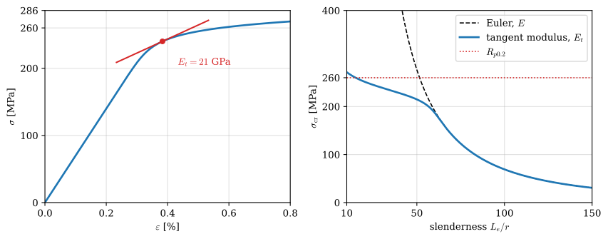
To make the procedure concrete we take an aluminium alloy with \(E = 70~\text{GPa}\) and \(R_{p0.2} = 260~\text{MPa}\), and describe its stress-strain curve with the Ramberg-Osgood form

\[ \varepsilon = \frac{\sigma}{E} + 0.002\left(\frac{\sigma}{R_{p0.2}}\right)^n \qquad\Rightarrow\qquad E_t = \left[\frac{1}{E} + \frac{0.002\,n}{R_{p0.2}}\left(\frac{\sigma}{R_{p0.2}}\right)^{n - 1}\right]^{-1} \]

with the exponent \(n = 20\) chosen for illustration. The plastic term gives the strain \(0.002\) at \(\sigma = R_{p0.2}\), as the definition of the offset yield strength requires. For each slenderness, 8.18.9 is solved for \(\sigma\) with a root finder.

E_al, R_al, n_ro = 70e3, 260, 20                 # MPa, MPa, the Ramberg-Osgood exponent

eps_ro = lambda s: s/E_al + 0.002*(s/R_al)**n_ro
E_t = lambda s: 1/(1/E_al + 0.002*n_ro/R_al*(s/R_al)**(n_ro - 1))

def sigma_tangent(lam):
    """The root of @eq-tangent-modulus at the slenderness lam."""
    return brentq(lambda s: s - np.pi**2*E_t(s)/lam**2, 1.0, 2*R_al)

lam = np.linspace(10, 150, 300)
s_t = np.array([sigma_tangent(l) for l in lam])

fig, (ax1, ax2) = plt.subplots(1, 2, figsize=(9, 3.6))
s = np.linspace(0, 1.1*R_al, 300)
ax1.plot(100*eps_ro(s), s, color='C0', lw=2)
s0 = 240                                         # a point on the knee and its tangent
de = np.linspace(-0.0015, 0.0015, 2)
ax1.plot(100*(eps_ro(s0) + de), s0 + E_t(s0)*de, color='C3', lw=1.5)
ax1.plot(100*eps_ro(s0), s0, 'o', color='C3', ms=5)
ax1.text(100*eps_ro(s0) + 0.05, s0 - 35, rf'$E_t = {E_t(s0)/1e3:.0f}$ GPa', color='C3')
ax1.set_xlabel(r'$\varepsilon$ [%]')
ax1.set_ylabel(r'$\sigma$ [MPa]')
ax1.set_xticks([0, 0.2, 0.4, 0.6, 0.8])
ax1.set_yticks([0, 100, 200, 260, 286])
ax1.set_xlim(0, 0.8)
ax1.set_ylim(0, 1.1*R_al)
ax1.grid(True, alpha=0.4)

ax2.plot(lam, np.pi**2*E_al/lam**2, color='black', lw=1.2, ls='--', label='Euler, $E$')
ax2.plot(lam, s_t, color='C0', lw=2, label='tangent modulus, $E_t$')
ax2.axhline(R_al, color='C3', lw=1.2, ls=':', label=r'$R_{p0.2}$')
ax2.set_xlabel(r'slenderness $L_e/r$')
ax2.set_ylabel(r'$\sigma_{\mathrm{cr}}$ [MPa]')
ax2.set_xticks([10, 50, 100, 150])
ax2.set_yticks([0, 100, 200, 260, 400])
ax2.set_xlim(10, 150)
ax2.set_ylim(0, 400)
ax2.grid(True, alpha=0.4)
ax2.legend()
fig.tight_layout()
plt.show()

The two curves coincide for slender columns, where the critical stress lies on the straight part of the stress-strain curve, and part company near \(R_{p0.2}\), where the tangent modulus collapses. The tangent-modulus curve never crosses the yield strength by much, which removes the unphysical rise of Euler’s curve for short columns. For a material with a gradual knee, such as aluminium, the transition is smooth, and Figure 8.18.11 shows that a column of slenderness \(50\) already buckles well below Euler’s prediction. A finite element analysis with an elastic-plastic material model does the same computation for an arbitrary section and arbitrary supports.

Design of centrally loaded columns

Real columns carry less than the ideal theory predicts. They are slightly crooked from manufacture, the load is never perfectly centred, and rolled and welded steel sections hold residual stresses from cooling that make parts of the section yield early. Each of these effects acts like the eccentricity of 8.18.8 and makes the column bend before it buckles. Design codes therefore do not use 8.18.3 or 8.18.9 directly. They use column curves calibrated against full-scale tests, and divide the column range into three parts: short columns, which fail by yielding, long columns, which follow Euler’s curve, and intermediate columns, for which an empirical curve bridges the two. In allowable stress design the critical stress from such a curve is divided by a factor of safety \(\Omega\),

\[ \sigma_{\text{allow}} = \frac{\sigma_{\text{cr}}}{\Omega} \]

and load and resistance factor design applies a resistance factor \(\phi < 1\) in its place. The American AISC specification follows this pattern [3]. In Europe, and through Boverket’s regulations in Sweden, steel columns are designed with Eurocode 3 [5]. It writes the yield strength as \(f_y\) and measures slenderness relative to \(\lambda_1\), the slenderness at which Euler’s curve meets the yield strength,

\[ \bar\lambda = \sqrt{\frac{A f_y}{N_{\text{cr}}}} = \frac{L_e/r}{\lambda_1}, \qquad \lambda_1 = \pi\sqrt{\frac{E}{f_y}} \]

where \(N_{\text{cr}} = P_{\text{cr}}\) is Euler’s load. The column carries the fraction \(\chi\) of the load \(A f_y\) at which its section yields,

\[ \begin{aligned} \chi &= \frac{1}{\Phi + \sqrt{\Phi^2 - \bar\lambda^2}} \le 1 \\ \Phi &= \frac{1}{2}\left[1 + \alpha_{\text{imp}}(\bar\lambda - 0.2) + \bar\lambda^2\right] \end{aligned} \tag{8.18.10}\]

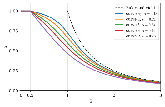
and its design resistance is \(N_{b,\text{Rd}} = \chi A f_y/\gamma_{M1}\) with the partial factor \(\gamma_{M1}\), recommended as \(1.0\). The imperfection factor \(\alpha_{\text{imp}}\) selects one of five curves, \(0.13\), \(0.21\), \(0.34\), \(0.49\) and \(0.76\) for the curves \(a_0\), \(a\), \(b\), \(c\) and \(d\). The code assigns a curve to each kind of section by how strongly its residual stresses and imperfections reduce its strength: a hot-finished hollow section in ordinary steel uses curve \(a\), a rolled I-section buckling about its weak axis curve \(b\) or \(c\), a welded box section curve \(b\), or \(c\) with thick welds, and a cold-formed tube curve \(c\).

def chi_ec3(lam_bar, a_imp):
    """The reduction factor of @eq-ec3-chi, with chi = 1 on the plateau lam_bar <= 0.2."""
    Phi = 0.5*(1 + a_imp*(lam_bar - 0.2) + lam_bar**2)
    return np.minimum(1/(Phi + np.sqrt(Phi**2 - lam_bar**2)), 1.0)

lb = np.linspace(0, 3, 300)
fig, ax = plt.subplots(figsize=(6, 3.8))
ax.plot(lb, np.minimum(1, 1/np.maximum(lb, 1e-9)**2), color='black', lw=1.2, ls='--',
        label=r'Euler and yield')
for name, a_imp, c in (('$a_0$', 0.13, 'C0'), ('$a$', 0.21, 'C1'), ('$b$', 0.34, 'C2'),
                       ('$c$', 0.49, 'C3'), ('$d$', 0.76, 'C4')):
    ax.plot(lb, chi_ec3(lb, a_imp), color=c, lw=2, label=rf'curve {name}, $\alpha = {a_imp}$')
ax.set_xlabel(r'$\bar\lambda$')
ax.set_ylabel(r'$\chi$')
ax.set_xticks([0, 0.2, 1, 2, 3], ['0', '0.2', '1', '2', '3'])
ax.set_yticks([0, 0.25, 0.5, 0.75, 1])
ax.set_xlim(0, 3)
ax.set_ylim(0, 1.1)
ax.grid(True, alpha=0.4)
ax.legend(fontsize=9)
plt.show()

The largest reduction compared with the ideal theory falls at \(\bar\lambda \approx 1\), where Euler’s curve and the yield strength meet. There the ideal column would carry its full squash load, while a real column with curve \(c\) carries about half of it. Imperfections matter most for columns of intermediate slenderness.

Example 1: A steel strut

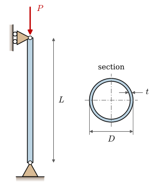
A pin-ended strut is made from a hot-finished circular hollow section \(60.3 \times 4.0\) (outer diameter \(D = 60.3~\text{mm}\), wall thickness \(t = 4.0~\text{mm}\)) in steel S355, with \(E = 210~\text{GPa}\) and \(f_y = 355~\text{MPa}\). Figure 8.18.13 shows it under the axial load \(P\). Determine Euler’s critical load, the squash load and the design resistance by Eurocode 3 for the lengths \(L = 1.5~\text{m}\) and \(L = 3.0~\text{m}\).

Both ends are pinned, so \(L_e = L\). The tube has the inner diameter \(d = D - 2t\) and the section properties

\[ A = \frac{\pi}{4}\left(D^2 - d^2\right), \qquad I = \frac{\pi}{64}\left(D^4 - d^4\right), \qquad r = \sqrt{\frac{I}{A}} \]

and for each length the slenderness \(\lambda = L/r\), Euler’s load \(N_{\text{cr}} = \pi^2 EI/L^2\), the squash load \(N_{\text{pl}} = A f_y\), the relative slenderness \(\bar\lambda = \sqrt{N_{\text{pl}}/N_{\text{cr}}}\) and, with curve \(a\) (\(\alpha_{\text{imp}} = 0.21\)) and \(\gamma_{M1} = 1.0\), the resistance \(N_{b,\text{Rd}} = \chi N_{\text{pl}}\) from 8.18.10.

D_t, t_t = 60.3, 4.0                     # mm
d_t = D_t - 2*t_t
E_s, f_y, gamma_M1 = 210e3, 355, 1.0     # MPa

A_t = np.pi/4*(D_t**2 - d_t**2)
I_t = np.pi/64*(D_t**4 - d_t**4)
r_t = np.sqrt(I_t/A_t)

ltx(r"A =", A_t, r"~\text{mm}^2, \quad I =", I_t/1e3, r"\cdot 10^3~\text{mm}^4, \quad r =", r_t,
    r"~\text{mm}", precision=4)

def strut(L_s):
    lam_s = L_s/r_t
    N_cr = np.pi**2*E_s*I_t/L_s**2/1e3                 # kN
    N_pl = A_t*f_y/1e3
    lam_bar = np.sqrt(N_pl/N_cr)
    chi = chi_ec3(lam_bar, 0.21)
    return lam_s, N_cr, N_pl, lam_bar, chi, chi*N_pl/gamma_M1

rows = []
for L_s in (1500, 3000):
    lam_s, N_cr, N_pl, lam_bar, chi, N_b = strut(L_s)
    rows.append(rf"L = {L_s/1e3:.1f}~\text{{m}}: &\quad \lambda = {lam_s:.0f}, \quad "
                rf"N_{{\text{{cr}}}} = {N_cr:.0f}~\text{{kN}}, \quad N_{{\text{{pl}}}} = {N_pl:.0f}~\text{{kN}}, "
                rf"\\ &\quad \bar\lambda = {lam_bar:.2f}, \quad \chi = {chi:.2f}, \quad "
                rf"N_{{b,\text{{Rd}}}} = {N_b:.0f}~\text{{kN}}")
ltx(r" \\ ".join(rows), aligned=True)

The short strut has \(\bar\lambda \approx 1\), the point of Figure 8.18.12 where the imperfections matter most. Euler’s load and the squash load are both about \(255~\text{kN}\), and either one alone would suggest that the strut carries that much, yet the code allows only two thirds of it. The long strut is clearly in the elastic range, Euler’s load is a quarter of that of the short one, and the code allows about \(90~\%\) of it. Doubling the length cut the resistance to a third, while the strength of the steel matters little: a steel of higher grade would raise the resistance of the short strut somewhat and that of the long strut hardly at all. A section with a larger radius of gyration, a tube of larger diameter and thinner wall, is the effective remedy.

Eccentric loads in design

When the load is known to be eccentric, the column carries an axial force and a bending moment at once. The secant formula 8.18.8 is exact for the ideal column with end eccentricity, but it is nonlinear in the load and awkward to use for design. Codes therefore check a linear interaction formula that adds the fraction of the allowable axial stress used by \(P/A\) to the fraction of the allowable bending stress used by \(Mc/I\),

\[ \frac{P/A}{\sigma_{a,\text{allow}}} + \frac{Mc/I}{\sigma_{b,\text{allow}}} \le 1 \tag{8.18.11}\]

where \(\sigma_{a,\text{allow}}\) is the allowable column stress for the slenderness of the member, from a column curve, and \(\sigma_{b,\text{allow}}\) the allowable bending stress [3]. Neither term may use up the whole capacity on its own, and the sum may not exceed one. Eurocode 3 uses the same structure with additional factors that amplify the moment for the extra bending caused by the deflection, the effect that 8.18.7 describes.

Buckling and the finite element method

The determinant condition that produced the critical loads above has a discrete counterpart. In a finite element model the axial forces add a geometric stiffness \(\bm K_G\) to the ordinary stiffness matrix \(\bm K\). It describes how the forces turn as the elements rotate, the effect we captured in every free body by taking moments in the deformed position. The model buckles at the load factor \(\lambda_{\text{b}}\) that makes the combined stiffness singular,

\[ \left(\bm K + \lambda_{\text{b}}\bm K_G\right)\bm\phi = \bm 0 \]

an eigenvalue problem whose smallest eigenvalue multiplies the applied load to give the critical load, and whose eigenvector \(\bm\phi\) is the buckling mode. Most solvers offer this linear buckling analysis, LS-DYNA with the keyword *CONTROL_IMPLICIT_BUCKLE. Like Euler’s formula, it assumes a perfect structure and an elastic material, and it predicts a load the real structure will not reach. A nonlinear analysis follows the load-deflection path instead, starting from a geometry given a small imperfection, often shaped like the first buckling mode, with large deflections and plasticity included, and finds the load at which the structure collapses.

The finite element method also covers the forms of buckling this chapter has left out. A beam bent about its strong axis can buckle sideways and twist, lateral-torsional buckling. The thin walls of a tube or a channel can buckle locally in short waves long before the member as a whole does, and thin shells such as cans and tanks are among the most imperfection-sensitive structures known. Local buckling is not always a failure to be avoided. The crash boxes behind a car bumper are thin-walled tubes designed to fold in a sequence of local buckles, and the energy they absorb while folding is what protects the rest of the structure in a collision.

Further reading

Hibbeler’s chapter 13 covers the same ground with many worked examples [3]. Euler’s memoir of 1757 is available in a scanned original [1], and Timoshenko’s memoir on the stability of elastic systems carries the energy method of this chapter further, to plates and other structures [6].